Robust and Accelerated PCA
Singular value decomposition and principal component analysis are powerful tools for finding low-rank representations of data matrices. However, many data matrices are only approximately low-rank, for example as a result of measurement errors, artifacts, or other nonlinear influences on the data acquisition process. In this section, we, therefore, want to discuss a PCA-variant that is robust towards outliers in the data. Before we introduce the method, we want to reformulate the problem of finding a low-rank approximation first.
Wright et al. defined Robust PCA (RPCA) as a decomposition of an $X \in \mathbb{R}^{n\times s}$ into the sum of two ${n\times s}$ components: a low-rank component $L$ and sparse component $S$. Namely, a convex optimization problem was defined as identifying the matrix components of $X=L+S$ that minimize a linear combination of the nuclear norm of $L$ and the L1-norm of $S$ such that $S \in \mathbb{R}^{n\times s}$ and $L \in \mathbb{R}^{n\times s}$. The motivation for such a decomposition is the fact that low-rank matrices are associated with a general pattern (e.g., the correct data in a corrupted dataset, a face in facial recognition), whereas a sparse matrix is connotated with disturbances (e.g., corrupted data values, effects, or shading of facial recognition).
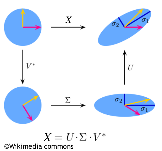
The problem of finding a low-rank matrix approximation $\hat{L}\in \mathbb{R}^{n\times s}$ to a (centered) matrix $X\in \mathbb{R}^{n\times s}$ (of potentially full rank) can be formulated as the optimization problem (for clarity, read first my post about SVD) can be depicted alternatively as
$$\hat{L}=\underset{L, S}{\arg \min } \left\{\frac{1}{2} \| S\| _{\text{Fro}}^2+\alpha \| L\| _*\right\} \,\,\,\,\,(1) $$
To make reader more familiar with the advantages of RPCA it is worth to look at RPCA using analogies. Imagine you are a detective trying to solve a case where important documents have been partially damaged by water, rendering some of the information unreadable. To make sense of the information and find patterns, you need a method that can help you fill in the gaps and extract useful information from the remaining text. This is where Robust PCA (RPCA) shines.
RPCA is advantageous in situations like this because it can separate the useful information (the low-rank component) from the damaged or missing parts (the sparse component). In our analogy, the low-rank component corresponds to the undamaged text, which follows a general pattern, while the sparse component represents the water damage, which affects only a small fraction of the text randomly. By separating the two components, RPCA allows you to focus on the undamaged text and extract valuable insights from it.
Another analogy would be to think of a photograph with random noise or scratches. The low-rank component represents the original, clean image, while the sparse component captures the noise and scratches. By decomposing the photograph into these two components, RPCA can help you recover the original, clean image and discard the unwanted noise.
In summary, RPCA is advantageous because it can handle situations where data is not strictly low-rank but instead is corrupted by sparse noise or errors. By separating the low-rank and sparse components, RPCA enables more accurate pattern recognition and data analysis, even in the presence of outliers and noise.
Here, $\| \cdot \| _*$ is the so-called nuclear norm, which is the one-norm of the vector of singular values of $X$, which is simply the sum of singular values, i.e.
$$\| L\| _*=\sum _{j=1}^{\min (n,s)} \sigma _j$$
where $\left\{\sigma _j\right\}_{j=1}^{\min (n,s)}$ denotes the singular values of $L$, and $\alpha > 0$ is the regularization parameter (to control the sparsity of the singular values of $L$). Thus, if we want to minimize (1), the $\| \cdot \| _*$ produces a sparse solution in terms of the singular values, namely the obtained matrix with many singular values reduced to zeros, and hence the rank of $L$ is automatically lower than the rank of $X$.
Problem (1) will find a matrix $\hat{L}$ close to $X$, with a lower rank, depending on the choice of $\alpha$. If $X$, however, is only low-rank up to some sparsely distributed but significant outliers, model (1) is not suitable for the approximation of this low-rank matrix. We, therefore, replace the squared Frobenius-norm in (1) with the matrix one-norm, i.e., $\| \cdot \| _1\text{:=}\sum _{j=1}^n \sum _{i=1}^s \left| \cdot _{\text{ij}}\right|$ , and obtain
$$\hat{L}=\underset{L,\,S}{\arg \min }\left\{\alpha \| L\| _*+\| S\| _1\right\}\,\,\,\,\,(2) $$
$$\hat{L}=\underset{L\in \mathbb{R}^{n\times s}, S\in \mathbb{R}^{n\times s}}{\arg \min }\left\{\alpha \| L\| _*+\| X - L\| _1\right\}\,\,\,\,\,(3) $$
If we substitute $S=X-L$ in (3), we obtain the problem in the form of the Robust PCA (RPCA) that will have to solve by optimisation $$\bm{\left(\hat{L},\hat{S}\right)=\,\,\, \underset{L\in \mathbb{R}^{n\times s},S\in \mathbb{R}^{n\times s}}{\arg \min } \left\{\| S\| _1+\alpha \| L\|_*\,\, \text{subject}\,\, \text{to}\,\, X=L+S\right\}\,\,\,\,(4)}$$
Note that $S$ refers to, for example, outliers, i.e., it represents the difference between our original data matrix $X$ and the low-rank matrix $L$.
(4) is our formulation of RPCA which we address here.
Problem (1) is a proximal mapping. There is the definition of the proximal mapping of function $f$, as a constraining regulizer, in context of the EU norm
$$prox_{f}(y)=\underset{x}{\arg \min }\left\{f(x)+\frac{1}{2} \| x-y\| _{2}^{2}\right\}$$
Let's show that our proximal mapping (1) has a simple closed form solution. In order to do so, note that for $R(L) =\|L\|_*$ we can guarantee $R(Q_1 L Q_2)=R(L)$ for two orthogonal matrices $Q_1 \in \mathbb{R}^{n\times n}$ and $Q_2 \in \mathbb{R}^{s\times s}$, which we see immediately from the observation that the SVD of $Q_1 L Q_2$ is the same as the SVD of $L$. In more details, we can discuss the property of the nuclear norm (i.e., $R(L) = |L|_*$) with respect to orthogonal matrices. The nuclear norm is invariant under orthogonal transformations, which means that for two orthogonal matrices $Q_1 \in \mathbb{R}^{n\times n}$ and $Q_2 \in \mathbb{R}^{s\times s}$, we have:
$$R(Q_1LQ_2)=R(L)$$
This property holds because the SVD of $Q_1 L Q_2$ is the same as the SVD of $L$. Let $L = U \Sigma V^T$ be the SVD of $L$. Then, the SVD of $Q_1 L Q_2$ can be obtained as:
$$Q_1LQ_2=(Q_1U)\Sigma (Q_2V)^T$$
Here, $(Q_1 U)$ and $(Q_2 V)$ are orthogonal matrices as the product of orthogonal matrices is also orthogonal. Since the nuclear norm is the sum of the singular values, and the singular values of $Q_1 L Q_2$ are the same as those of $L$, we have:
$$R(Q_1LQ_2)=\sum_{j=1}^{\min(n,s)}\sigma_j = \sum_{j=1}^{\min(n,s)}\sigma_j=R(L)$$
This property of the nuclear norm being invariant under orthogonal transformations holds true. However, it is important to note that this property does not directly relate to the problem (1) or the proximal mapping as presented in the original passage. Instead, it provides a useful insight into the properties of the nuclear norm, which can be helpful in understanding the behavior of the optimization problem (1) and the proximal mapping.
If $X=U \Sigma V^T$ denotes the SVD of X, we can substitute $\hat{L}$ for $\hat{L}=U \hat{L} V^T$ with
$$\hat{L}=\underset{L\in \mathbb{R}^{n\times s}}{\arg \min }\left\{\frac{1}{2}\| ULV^T-U \Sigma V^T\|_{Fro}^2 + \alpha \|U L V^T\| _* \right\}=\underset{L\in \mathbb{R}^{n\times s}}{\arg \min }\left\{\frac{1}{2}\| L- \Sigma\|_{Fro}^2 + \alpha \| L \| _* \right\}\,\,\,\,\,(5) $$
Since $\Sigma$ is a diagonal matrix with non-negative entries, the solution (5) has to be a diagonal matrix with non-negative entries, too. As a result, (5) simplifies to
$$\hat{l}=\underset{L\in \mathbb{R}^{min(n,s)}_{\geq 0}}{\arg \min }\left\{\frac{1}{2}\| l- \sigma \|^2 + \alpha \sum _{j=1}^{\min (n,s)} l_j\right\}=\underset{L\in \mathbb{R}^{min(n,s)}_{\geq 0}}{\arg \min }\left\{\frac{1}{2}\sum _{j=1}^{\min (n,s)} \left(l_j-\sigma _j\right){}^2 + \alpha \sum _{j=1}^{\min (n,s)} l_j\right\}\,\,\,\,\,(6) $$
where $l \in \mathbb{R}^{min(n,s)}_{\geq 0}$ is the vector of diagonal entries of $\hat{L}$, i.e. $\hat{L}=diag(l)$, and also the vecor of singular values of $\hat{L}$. The vector $\sigma \in \mathbb{R}^{min(n,s)}_{\geq 0}$ denotes singular values of $\Sigma$, i.e. $\Sigma=diag(\sigma)$ .
The problem (6) has the closed-form solution in the form of soft-thresholding of the singular values $\sigma$. Hence, we observe
$$\hat{l}_j = max(\sigma_j - \alpha, 0), \,\,\, \forall j \in \{1,\text{...},\min (n,s)\} $$
We can therefore compute the solution of (1) via
$$ \hat{L}=U \hat{L} V^T,\,\,\,\, \forall \,\,\, \hat{L}=diag(\hat{l})$$
For our data matrix $ X=U\Sigma V^T,$, the above can be written in the proximal notation as
$$\hat{L}=(I+\alpha\, \partial \| \cdot \| _* )^{-1}(X)=\,U\,\,\text{diag}\left(\text{soft}_{\alpha} (\sigma)\right)V^T,\,\,\,\,\,\, \text{soft}_{\alpha}(\sigma)_j = \begin{cases} \sigma_j-\alpha & \text{: }\,\, \sigma_j>\alpha \\ 0 & \text{: }\,\,\, other \end{cases} ,\,\,\,\,\,\,\,\,\,\,(7)$$
The practical implications of this proximal map are as follows. Given a matrix $X$, all singular values below threshold $\alpha$ will be set to zero, therefore enforcing a lower rank $\hat{L}$ compared to $X$ if $\alpha$ is larger than at least the smallest singular value of $X$. All other singular values are reduced by the factor $\alpha$.
We can derive the closed-form solution for the proximal mapping of the nuclear norm from $(I+\alpha, \partial | \cdot |_* )^{-1}(X)$ to $U\,\text{diag}\left(\text{soft}_{\alpha} (\sigma)\right)V^T$ as follows:
I. Start with the proximal mapping of the nuclear norm for a given matrix $X$:
$$\hat{L} = (I + \alpha\, \partial \| \cdot \|_*)^{-1}(X)$$
II. Using the SVD of $X$, we can represent $X$ as $X = U \Sigma V^T$. Then, the proximal mapping becomes:
$$\hat{L} = (I + \alpha\, \partial \| \cdot \|_*)^{-1}(U \Sigma V^T)$$
III. Since the nuclear norm is unitarily invariant, we can directly apply the proximal operator on the singular values $\sigma$ in the diagonal matrix $\Sigma$. The proximal mapping simplifies to:
$$\hat{L} = U\, (I + \alpha\, \partial \| \cdot \|_*)^{-1}(\Sigma) V^T$$
IV. Now, we can find the closed-form solution for the proximal operator applied to the singular values in $\Sigma$. This is given by the soft-thresholding function:
-
Start from the equation in III, $\hat{L} = U\, (I + \alpha\, \partial \| \cdot \|_*)^{-1}(\Sigma) V^T$.
-
We know that $(I + \alpha, \partial | \cdot |_*)^{-1}(\Sigma)$ is the proximal mapping applied to the diagonal matrix $\Sigma$. To obtain the closed-form solution, we need to minimize the following objective function, where $\| \cdot \|_{Fro}$ denotes the Frobenius norm and $\| \cdot \|_*$ denotes the nuclear norm: $$\min_L \frac{1}{2} \| L - \Sigma \|_{Fro}^2 + \alpha \| L \|_*$$
-
We can rewrite the nuclear norm as the sum of the singular values: $$\| L \|_* = \sum_{i=1}^{\min(n,s)} \sigma_i(L)$$
-
Since $L$ and $\Sigma$ are diagonal matrices, we can express the Frobenius norm as the sum of squared differences between their diagonal elements: $$\| L - \Sigma \|_{Fro}^2 = \sum_{i=1}^{\min(n,s)} (\sigma_i(L) - \sigma_i(\Sigma))^2$$
-
Now, we can rewrite the objective function in terms of the singular values: $$\min_L \frac{1}{2} \sum_{i=1}^{\min(n,s)} (\sigma_i(L) - \sigma_i(\Sigma))^2 + \alpha \sum_{i=1}^{\min(n,s)} \sigma_i(L)$$
-
We can solve this optimization problem element-wise by minimizing the following function for each singular value: $$\min_{\sigma_i(L)} \frac{1}{2} (\sigma_i(L) - \sigma_i(\Sigma))^2 + \alpha \sigma_i(L)$$
-
Taking the derivative with respect to $\sigma_i(L)$ and setting it to zero, we get: $$ (\sigma_i(L) - \sigma_i(\Sigma)) + \alpha = 0 $$
-
Solving for $\sigma_i(L)$, we find the soft-thresholding function: $$ \sigma_i(L) = \sigma_i(\Sigma) - \alpha $$
-
However, since singular values are non-negative, we need to enforce the non-negativity constraint: $$ \sigma_i(L) = \begin{cases} \sigma_i(\Sigma) - \alpha & \text{if } \sigma_i(\Sigma) > \alpha \\ 0 & \text{otherwise} \end{cases} $$
V. Now, we can substitute the soft-thresholding function back into the expression for $\hat{L}$:
Since we now have the optimal solution for each singular value $\sigma_i(L)$, we can substitute these values back into the expression for the proximal mapping. The term $(I + \alpha\, \partial \| \cdot \|_*)^{-1}(\Sigma)$ represents the proximal operator applied to the singular values in $\Sigma$. We have found that the optimal solution for the singular values is given by the soft-thresholding function. Therefore, we can replace $(I + \alpha\, \partial \| \cdot \|_*)^{-1}(\Sigma)$ with a diagonal matrix containing the soft-thresholded singular values, which we denote as $\text{diag}(\text{soft}_\alpha(\sigma))$: $$ \hat{L} = U\, \text{diag}(\text{soft}_\alpha(\sigma)) V^T $$
VI. We have now substituted the soft-thresholded singular values back into the expression for the proximal mapping. This final expression gives us a closed-form solution for the proximal mapping of the nuclear norm, using the SVD of $X$ and the soft-thresholding function applied to the singular values.
$$ \hat{L} = U\, \text{diag}(\text{soft}_\alpha(\sigma)) V^T $$
$$ \text{soft}_{\alpha}(\sigma)_j = \begin{cases} \sigma_j-\alpha & \text{if }\,\, \sigma_j>\alpha \\ 0 & \text{otherwise} \end{cases}$$
$$\,\,\,\,\,\,\,\,\,\,\,\,\,\,\,\,\,\,\,\,\,\,\,\,\,\,\,\,\,\,\,\,\,\,\,\,\,\,\,\,\,\,\,\,\,\,\,\,\,\,\,\,\,\,\,\,\,\,\,\,\,\,\,\,\,\,\,\,\,\,\,\,\,\,\,\,\,\,\,\,\,\,\,\,\,\,\,\,\,\,\,\,\,\,\,\,\,\,\,\,\,\,\,\,\,\,\,\,\,\,\,\,\,\,\,\,\,\,\,\,\,\,\,\,\,\,\,\,\,\,\,\,\,\,\,\,\,\,\,\,\,\,\,\,\,\,\,\,\,\,\,\,\,\,\,\,\,\,\,\,\,\,\,\,\,\,\,\,\,\,\,\,\,\,\,\,\,\,\,\,\,\,\,\,\,\,\,\,\,\,\,\,\,\,\,\,\,\,\,\,\,\,\,\,\,\,\,\,\,\,\,\,\,\,\,\,\,\,\,\,\,\,\,\,\,\,\,\,\,\,\,\,\,\,\,\,\,\,\,\,\,\,\,\,\,\,\,\,\,\,\,\,\,\,\,\,\,\,\,\,\,\,\,\,\,\,\,\,\,\,\,\,\,\,\,\,\,\,\,\,\,\,\,\,\,\,\,\,\,\,\,\,\,\,\,\,\,\,\,\,\,\,\,\,\,\,\,\,\,\,\,\,\,\,\,\,\,\,\,\,\,\, \blacksquare $$
The VI. can be implemented for a given image as follows:
-
We start with the definition of the soft-thresholding function:
$$ \text{soft}_{\alpha}(\sigma)_j = \begin{cases} \sigma_j-\alpha & \text{if }\,\, \sigma_j>\alpha \\ 0 & \text{otherwise} \end{cases} $$
-
We can rewrite the soft-thresholding function by separating the conditions and the value of $\sigma_j$:
$$ \text{soft}_{\alpha}(\sigma)_j = \sigma_j - \alpha \cdot I_{\{\sigma_j>\alpha\}} $$
where $I_{\{\sigma_j>\alpha\}} = \begin{cases} 1 & \text{if } \sigma_j>\alpha \\ 0 & \text{otherwise} \end{cases}$ is the indicator function that equals 1 when the condition in the subscript is true and 0 otherwise. The indicator function essentially 'turns off' the subtraction of $\alpha$ when $\sigma_j \leq \alpha$.
-
The indicator function can be rewritten as the positive part of the signum function applied to $\sigma_j - \alpha$. The signum function, sign(x), returns -1 if x < 0, 0 if x = 0, and 1 if x > 0. Thus, the positive part of sign($\sigma_j - \alpha$) equals 1 if $\sigma_j > \alpha$ and 0 otherwise:
$$ \text{soft}_{\alpha}(\sigma)_j = \sigma_j - \alpha \cdot \max\{0, \text{sign}(\sigma_j - \alpha)\} $$
-
Now, we can rewrite the expression inside the max function using absolute values. The expression $\sigma_j - \alpha$ is positive when $\sigma_j > \alpha$ and negative otherwise. So, the absolute value of this expression equals $\sigma_j - \alpha$ when $\sigma_j > \alpha$ and $\alpha - \sigma_j$ when $\sigma_j \leq \alpha$. This allows us to rewrite the max function as follows:
$$ \text{soft}_{\alpha}(\sigma)_j = \sigma_j - \alpha \cdot \max\{0, \text{sign}(|\sigma_j - \alpha|)\} $$
-
Finally, we recognize that the right-hand side of this equation now has the form of the proximal operator of the $\ell_1$ norm, with $\tau = \alpha$ and $z = \sigma_j$:
$$ prox_{\tau}(\sigma_j) = \text{sign}(\sigma_j) \cdot \max\{0, |\sigma_j| - \tau\} $$
where $R$ represents the $\ell_1$ norm and $\tau = \alpha$ is the threshold parameter. This clearly shows the connection between the soft-thresholding operation and the proximal operator formulation. This reads "the proximal operator of the function, evaluated at $\sigma_j$, is equal to the sign of $\sigma_j$ times the maximum of 0 and the absolute value of $\sigma_j$ minus $\tau$".
This shows the detailed transformation from the soft-thresholding function to the proximal operator. Note that the soft-thresholding function is essentially the proximal operator of the $\ell_1$ norm, and it's applied element-wise to the singular values of a matrix in the context of nuclear norm minimization.
import matplotlib.pyplot as plt
import numpy as np
from skimage import data
def soft_threshold(x, alpha):
return np.sign(x) * np.maximum(np.abs(x) - alpha, 0)
def nuclear_norm_proximal(X, alpha):
# Perform singular value decomposition
U, sigma, Vt = np.linalg.svd(X, full_matrices=False)
# Apply the soft-thresholding function to the singular values
sigma_soft = soft_threshold(sigma, alpha)
# Compute the proximal mapping of the nuclear norm
L = U @ np.diag(sigma_soft) @ Vt
return L
# Load the image
image1 = data.astronaut()
# Normalize the image
image1_normalized = image1 / 255.0
# Separate color channels
R, G, B = image1_normalized[:, :, 0], image1_normalized[:, :, 1], image1_normalized[:, :, 2]
# Define a list of alpha values
alphas = [10, 7.5, 5, 2, 0.1]
# Create a subplot for the original image
plt.figure(figsize=(18, 10))
plt.subplot(2, 3, 1)
plt.imshow(image1)
plt.title('Original RGB Image')
plt.axis('off')
# Iterate through the alpha values and create subplots for each low-rank approximation
for i, alpha in enumerate(alphas, 2):
R_approx = nuclear_norm_proximal(R, alpha)
G_approx = nuclear_norm_proximal(G, alpha)
B_approx = nuclear_norm_proximal(B, alpha)
# Combine approximated color channels into a single RGB image
approx_image = np.stack((R_approx, G_approx, B_approx), axis=2)
approx_image = np.clip(approx_image, 0, 1)
plt.subplot(2, 3, i)
plt.imshow(approx_image)
plt.title(f'Low-rank Approximation ($\\alpha$={alpha})')
plt.axis('off')
plt.tight_layout()
plt.show()

The np.clip function is necessary because the nuclear norm proximal operation applied to the color channels of the image might produce values that are outside the valid range for pixel intensities, which are between 0 and 1 for normalized images. np.clip ensures that all values in the approximated image lie within this range, by setting any values below 0 to 0 and any values above 1 to 1. This prevents issues with displaying the image or saving it in an incorrect format.
In the provided code, the different values of $\alpha$ produce different levels of approximation, with larger $\alpha$ values resulting in more aggressive approximations. As you can see in the generated subplots, higher $\alpha$ values result in more noticeable artifacts and simplification of the image, while lower $\alpha$ values produce approximations that are visually closer to the original image.
In summary, the proximal mapping of the nuclear norm is useful in various low-rank optimization problems, such as matrix completion, robust PCA, and collaborative filtering. In these problems, we want to find a low-rank matrix that best approximates the given data while being consistent with certain constraints.
The closed-form solution for the proximal mapping, $\hat{L} = U \text{diag}\left(\text{soft}_{\alpha} (\sigma)\right) V^T$, allows for efficient computation in optimization algorithms, such as proximal gradient methods or accelerated proximal gradient methods. These algorithms are used to solve problems involving a smooth loss function plus a nonsmooth regularization term, like the nuclear norm.
The soft-thresholding function, $\text{soft}_{\alpha}(\sigma)_j$, applies element-wise shrinkage to the singular values of the matrix. This operation promotes sparsity in the singular values, which is equivalent to promoting a low-rank structure in the matrix. The parameter $\alpha$ controls the amount of shrinkage applied to the singular values, and it can be tuned according to the specific problem and desired low-rank structure.
Derivtion of algorithm for the numerical solution of (4) - The Linearised Bregman Iteration for Robust PCA (RPCA) 
For the preliminaries, note that the mapping $(I+\tau \partial R )^{-1}:C\rightarrow C$, where C is a convex set, is known as the proximal operator w.r.t $R$ here. Remember also that when we derive gradient descent, we always choose function $J(w) := \frac{1}{2\tau} |w|^2$. As a result, we minimise gradient of function $E$ plus the subgradient of $R$, and $q$ is a subgradient in $R$. We base our algorithm on so-called Bregman iteration
$$w^{(k+1)}=\underset{w\in \mathbb{R}^{n}}{\arg \min }\left\{E(w)+D_j^{p^k}\left(w,w^k\right) \right\}\,\,\,\,\,(8a)$$
$$p^{k+1}=p^k-\nabla E(w^{k+1})\,\,\,\,\,(8b)$$
for inituial values $w^0$ and $p^0 \in \partial J(w^0)$, where $\partial J$ denotes the subdifferential of $J$ and $D^p_J(w, v)$ is the generalised Bregman distance
$$D^p_J(w, v)=J(w)-J(v)-\langle p,w-v\rangle$$
The Bregamn divergence is the difference between value $J(w)$ and value of the hyperplane $J(v)-\nabla J(v)(w-v)$, but in the above the gradient is replaced by the subgradient $p \in \partial J(v)$. Note, that we know that both $\| \cdot \| _*$ and $\| \cdot \| _1$ are not differentiable, but are still convex, and so the subgradient is useful. As for the original Bregman method, we can obtain a linearised variant for the choice $J(w)=\frac{1}{\tau}(\frac{1}{2}\|w\|^2+R(w))-E(w)$. After pluging in $J(w):=\frac{1}{2}\tau \| w \|^2$, the method (8) and performing steps
- Begin with the original Bregman iteration method, (8a), and plug in the specific form of $J(w)$: $$ w^{(k+1)} = \underset{w\in \mathbb{R}^{n}}{\arg \min }\left\{E(w) + \frac{1}{2}\tau\|w\|^2 - \frac{1}{2}\tau\|w^k\|^2 - p^k(w-w^k) \right\} $$
- Now, plug in the definition of the Bregman distance, $D_{J}^{p^k}(w, w^k)$: $$ w^{(k+1)} = \underset{w\in \mathbb{R}^{n}}{\arg \min }\left\{E(w) + D_{J}^{p^k}(w, w^k)\right\} $$
- Substitute $J(w):=\frac{1}{2}\tau \| w \|^2$: $$ w^{(k+1)} = \underset{w\in \mathbb{R}^{n}}{\arg \min }\left\{E(w) + \frac{\tau}{2} (w^2 - w^{k^2}) - p^k(w - w^k)\right\} $$
- Rearrange the terms and complete the square: $$ w^{(k+1)} = \underset{w\in \mathbb{R}^{n}}{\arg \min }\left\{\frac{1}{2}\| w - (w^k - \tau \nabla E(w^k))\|^2 + p^k(w - w^k) - \frac{1}{2}\tau\|w^k\|^2 + E(w^k)\right\} $$
- Observe that the minimization problem on the right-hand side is equivalent to minimizing the sum of a squared Euclidean distance term and the Bregman distance $D_R^{q^k}(w,w^k)$: $$ w^{(k+1)} = \underset{w\in \mathbb{R}^{n}}{\arg \min }\left\{\frac{1}{2}\| w - (w^k - \tau \nabla E(w^k))\|^2 + D_R^{q^k}(w,w^k)\right\} $$
- Next, notice that the proximal operator of the mapping $(I+\tau\, \partial R)^{-1}$ can be applied to simplify this expression: $$ w^{(k+1)} = (I+\tau\, \partial R)^{-1}(q^k-\tau \nabla E(w^k)+w^k) $$
Now we have derived equation (9a) as below
$$ w^{k+1}=\underset{w\in \mathbb{R}^{n}}{\arg \min }\left\{ \frac{1}{2}\| w-\left(w^k-\tau \nabla E (w^k)\right)\|^2 + D_R^{q^k}\left(w,w^k\right) \right\}=(I+\tau\, \partial R )^{-1}(q^k-\tau \nabla E(w^k)+w^k)\,\,\,\,(9a)$$
To update subgradient we have to make
- Recall the update rule for the subgradient $p^{k+1}$: $$ p^{k+1} = p^k - \nabla E(w^{k+1}) $$
- We have the update rule for $w^{k+1}$ from equation (9a): $$ w^{k+1} = (I+\tau\, \partial R)^{-1}(q^k-\tau \nabla E(w^k)+w^k) $$
- Since we're updating the subgradient $q^{k+1}$, we need to relate $q^{k+1}$ to $p^{k+1}$. Note that, in this case, $p^k = q^k$. So, substitute $p^k$ with $q^k$ in the update rule for $p^{k+1}$: $$ q^{k+1} = q^k - \nabla E(w^{k+1}) $$
- Now, we need to express $\nabla E(w^{k+1})$ in terms of $w^k$, $q^k$, and other known quantities. To do this, we can rearrange the equation (9a) for $w^{k+1}$: $$ w^{k+1} - w^k = (I+\tau\, \partial R)^{-1}(q^k-\tau \nabla E(w^k)) - w^k $$
- From this, we can express $\nabla E(w^k)$ as: $$ \nabla E(w^k) = \frac{1}{\tau} (q^k - (I+\tau\, \partial R)(w^{k+1} - w^k)) $$
- Substitute this expression for $\nabla E(w^k)$ into the update rule for $q^{k+1}$: $$ q^{k+1} = q^k - \left(\frac{1}{\tau} (q^k - (I+\tau\, \partial R)(w^{k+1} - w^k))\right) $$
- Simplify the equation: $$ q^{k+1} = q^k - (w^{k+1} - w^k - \tau \nabla E(w^k)) $$ So, for subgradients $q^k \in \partial R(w^k)$ we enjoy $$q^{k+1}=q^k - (w^{k+1}-w^k-\tau \nabla E(w^k))\,\,\,\,\,(9b)$$
In the following, we want to focus on the special case $E(w)=\frac{1}{2}\|Aw-b\|^2$, for a matrix $A \in \mathbb{R}^{s \times n}$ and a vector $b \in \mathbb{R}^{s}$. For this special case we have gradient descent iterations for energy $E$, and the (9) reads
$$w^{k+1}=(I+\tau\, \partial R )^{-1}(w^k+q^k-\tau A^T(Aw^k-b))\,\,\,\,(10a)$$ $$q^{k+1}=q^k-(w^{k+1}+w^k-\tau A^T(Aw^k-b))\,\,\,\,(10b)$$
If we assume that $(w^k+q^q)/\tau \in R$, we can sabstitute $\tau A^T b^k = w^k+q^k-\tau A^T(Aw^k-b)$ which modifies (10) to
$$w^{k+1}=(I+\tau\, \partial R )^{-1}(\tau A^T b^k)\,\,\,\,(11a)$$ $$b^{k+1}=b^k-(Aw^{k+1}-b)\,\,\,\,(11b)$$
Let's go through the derivation from (10) to (11) more explicitly, including the substitution steps:
- Begin with the update rule (10a): $$w^{k+1}=(I+\tau\, \partial R )^{-1}(w^k+q^k-\tau A^T(Aw^k-b))$$
- Based on the assumption that $\frac{w^k + q^k}{\tau} \in \mathcal{R}(A^T)$, there exists a vector $b^k$ such that: $$\frac{w^k + q^k}{\tau} = A^T b^k$$
- Multiply both sides of this equation by $\tau$: $$w^k + q^k = \tau A^T b^k$$
- Now, substitute this expression for $\tau A^T b^k$ into the update rule for $w^{k+1}$: $$w^{k+1}=(I+\tau\, \partial R )^{-1}(w^k + q^k - \tau A^T(Aw^k - b))$$
- Notice that $w^k + q^k - \tau A^T(Aw^k - b) = \tau A^T b^k$. Replace the expression inside the parentheses: $$w^{k+1}=(I+\tau\, \partial R )^{-1}(\tau A^T b^k)$$ This gives us equation (11a).
- Now, move on to the update rule (10b): $$q^{k+1}=q^k-(w^{k+1}+w^k-\tau A^T(Aw^k-b))$$
- Recall the expression for $\tau A^T b^k$ obtained in step 3: $$w^k + q^k = \tau A^T b^k$$
- Substitute this expression into the update rule for $q^{k+1}$: $$q^{k+1}=q^k - (w^{k+1} - \tau A^T b^k + w^k)$$
- Recognize that $w^{k+1} = A(I+\tau\, \partial R )^{-1}(\tau A^T b^k)$, as obtained in step 5.
- Use this to rewrite the update rule for $b^{k+1}$: $$b^{k+1}=b^k-(Aw^{k+1}-b)$$ This gives us equation (11b).
In summary, we have obtained the modified update rules (11a) and (11b) from (10a) and (10b) by making the assumption that $\frac{w^k + q^k}{\tau} \in R(A^T)$ and making the appropriate substitutions:
$$w^{k+1}=(I+\tau\, \partial R )^{-1}(\tau A^T b^k)\,\,\,\,(11a)$$ $$b^{k+1}=b^k-(Aw^{k+1}-b)\,\,\,\,(11b)$$
with initial value $b^0=b$. Combining both equations into one
- Start with equation (11a): $$w^{k+1}=(I+\tau\, \partial R )^{-1}(\tau A^T b^k)$$
- Now, look at equation (11b): $$b^{k+1}=b^k-(Aw^{k+1}-b)$$
- Substitute the expression for $w^{k+1}$ from (11a) into (11b): $$b^{k+1}=b^k-(A(I+\tau\, \partial R )^{-1}(\tau A^T b^k)-b)$$ yields $$\bm{b^{k+1}=b^k-(A(I+\tau\, \partial R )^{-1}(\tau A^T b^k)-b)\,\,\,\,(12)}$$
The (12) is just gradient descent applied to a very specific energy that we characterise with the following lemma
Lemma Linearised Bregman iteration as gradient descent
First, it is necessary to mention about the Moreau-Yosida regularization of a function, here, $R$. It is a technique used to create a smooth approximation of the function. In the context of optimization problems, it can help in solving non-smooth or non-convex problems. Given a function $R: \mathbb{R}^n \to \mathbb{R}$, its Moreau-Yosida regularization $\tilde{R}(z)$ is defined as:
$$\tilde{R}(z) := \underset{x \in \mathbb{R}^n}{inf} \left\{ R(x)+\frac{1}{2} \|x-z\|^2 \right\}$$
It is a function that combines the original function $R(x)$ with a quadratic penalty term, $\frac{1}{2}|x-z|^2$. The resulting function $\tilde{R}(z)$ is a smoothed version of $R(x)$, which is more amenable to gradient-based optimization methods. Namely, we are minimizing the sum of the original function $R(x)$ and the quadratic penalty term $\frac{1}{2} |x - z|^2$. The quadratic term ensures that the resulting function $\tilde{R}(z)$ is strongly convex, which often leads to better convergence properties and stability when used in optimization algorithms.
By using the infimum, we are able to obtain the lowest possible value for the regularized function, even in cases where the minimum is not actually achieved. This is important in optimization because it allows us to find the best possible solution for a given problem, even when the problem is not well-behaved or has no unique solution.
The linearised Bregman iteration in the form (12) is a gradient descent with step-size one, i.e.
$$b^{k+1}=b^k - \nabla G_{\tau}(b^k)$$
applied to the energy
$$G_{\tau}(b^k) := \frac{\tau}{2}\|A^T b^k\|^2-\left\langle b^k,b\right\rangle -\frac{\tilde{R} \left( \text{$\tau $A}^T b^k\right)}{\tau}\,\,\,\,\,(13) $$
The choice of the function $G_{\tau}(b^k)$ is motivated by the desire to connect the Linearized Bregman iteration (LBI) with the gradient descent optimization framework. The goal is to rewrite the LBI updates in a form that resembles the gradient descent algorithm, which is known for its simplicity and wide applicability. The function $G_{\tau}(b^k)$ is chosen so that its gradient, when used as an update rule, is equivalent to the LBI update equation (12). Let's break down the components of $G_{\tau}(b^k)$:
- $\frac{\tau}{2}|A^T b^k|^2$: This term represents a quadratic function of $b^k$, and it is related to the energy function $E(w) = \frac{1}{2}|Aw - b|^2$. Taking the gradient of this term with respect to $b^k$ will produce a term involving $A^T(Aw^k - b)$, which appears in the LBI update.
- $-\left\langle b^k, b \right\rangle$: This term is a linear function of $b^k$. The gradient of this term with respect to $b^k$ is simply $-b$, which also appears in the LBI update.
- $-\frac{\tilde{R}(\tau A^T b^k)}{\tau}$: This term is the Moreau-Yosida regularization of the function $R$, scaled by a factor of $-\frac{1}{\tau}$. The gradient of this term will involve the proximal operator, connecting the LBI update with the structure of the regularization function.
Here $\tilde{R}(z)$ refers to the Moreau-Yosida regularisation of the function $R$, i.e.
$$\tilde{R} := \underset{x \in \mathbb{R}^n}{inf} \left\{ R(x)+\frac{1}{2} \|x-z\|^2 \right\}=R((I+\tau\, \partial R )^{-1}(z))+\frac{1}{2}\|(I+\tau\, \partial R )^{-1}(z)-z \|^2$$
or
$$\tilde{R}(z) = R(\text{prox}_{\tau R}(z)) + \frac{1}{2}\|\text{prox}_{\tau R}(z) - z\|^2$$
We start with the general form of the soft-thresholding operator:
$$ \text{prox}_{\tau R}(z) = \text{sign}(z) \cdot \max\{0, |z| - \tau\} $$
Now, let's consider the three cases based on the value of $z$:
- When $z > \tau$: $$ \text{prox}_{\tau R}(z) = \text{sign}(z) \cdot \max\{0, |z| - \tau\} = \text{sign}(z) \cdot (|z| - \tau) = z - \tau $$
- When $|z| \leq \tau$: $$ \text{prox}_{\tau R}(z) = \text{sign}(z) \cdot \max\{0, |z| - \tau\} = \text{sign}(z) \cdot 0 = 0 $$
- When $z < -\tau$: $$ \text{prox}_{\tau R}(z) = \text{sign}(z) \cdot \max\{0, |z| - \tau\} = \text{sign}(z) \cdot (|z| - \tau) = z + \tau $$
Combining these cases, we get the following piecewise function:
$$ \text{prox}_{\tau R}(z) = \begin{cases} z - \tau, & \text{if } z > \tau \\ 0, & \text{if } |z| \leq \tau \\ z + \tau, & \text{if } z < -\tau \end{cases} $$
The above claims that the linearized Bregman iteration in the form of equation (12) is equivalent to gradient descent applied to the energy function $G_{\tau}(b^k)$. This means that the update rule for $b^{k+1}$, as per equation (12), should match the gradient descent update rule $b^{k+1} = b^k - \nabla G_{\tau}(b^k)$.
If this is true, it implies that the linearized Bregman iteration can be interpreted as gradient descent applied to a specific energy function, and it may help in understanding the convergence properties and other aspects of the algorithm.
Here, $(I+\tau, \partial R)^{-1}(z)$ represents the proximal operator of the function $R$, which is applied to the input $z$. The proximal operator is a generalization of the gradient step in optimization algorithms and is particularly useful for non-smooth optimization problems. In this expression, the Moreau-Yosida regularization $\tilde{R}(z)$ is obtained by computing the proximal operator of $R$ applied to $z$ and adding a quadratic penalty term based on the difference between the proximal operator and the input $z$.
Proof
The proof is relatively straightforward if we compute the gradient $\tilde{R}$, since the gradient of $\frac{\tau}{2}\|A^T b^k \|^2-\langle b^k, b \rangle$ simple reads $\tau A^T A b^k-b$. in order to compute the gradient $\nabla \tilde{R}$, we first rewrite $\tilde{R}$ to
$$\tilde{R}(z) := \underset{x \in \mathbb{R}^n}{inf} \left\{ R(x)+\frac{1}{2} \|x-z\|^2 \right\}=$$ $$\,\,\,\,\,\,\,\,\,\,\,\,\,\,\,\,\,\,\,\,\,\,\,\,\,\,\,\,\,\,\,\,\,\,\,\,\,\,\,\,\,\,\,\,\,\,\,\,\,\,\,\,\,\,\, \underset{x \in \mathbb{R}^n}{inf} \left\{ R(x)+\frac{1}{2} \|x\|^2 - \langle x,z \rangle +\frac{1}{2}\|z\|^2 \right\}= $$ $$\,\,\,\,\,\,\,\,\,\,\,\,\,\,\,\,\,\,\,\,\,\,\,\,\,\,\,\,\,\,\,\,\,\,\,\,\,\,\,\,\,\,\,\,\,\,\,\,\,\,\,\,\,\,\, \frac{1}{2}\|z\|^2-\underset{x \in \mathbb{R}^n}{sup} \left\{\langle x,z \rangle- R(x)-\frac{1}{2} \|x\|^2 \right\}= $$ $$\,\,\,\,\,\,\,\,\,\,\,\,\,\,\,\,\,\,\,\,\,\,\,\,\,\,\,\,\,\,\,\,\frac{1}{2}\|z\|^2-(\frac{1}{2}\|\cdot\|^2+R )^*(z)\,\,\,\,(14)$$
The switch from infimum to supremum and the appearance of $\frac{1}{2}\|z\|^2$ outside the supremum are results of applying the Fenchel conjugate to the function inside the infimum. The Fenchel conjugate, also known as the Legendre-Fenchel transform or the convex conjugate, is a way to transform a convex function into its dual representation.
Given a function $f(x)$, its Fenchel conjugate is defined as:
$$F^*(y) = \underset{x}{\sup}\{\langle x, y \rangle - F(x)\}$$
Applying the Fenchel conjugate to the function inside the infimum, we get:
$$\tilde{R}(z) = \frac{1}{2}\|z\|^2 - \left(\frac{1}{2}\|\cdot\|^2 + R\right)^*(z)$$
Here, we have switched from infimum to supremum, and the $\frac{1}{2}\|z\|^2$ term has been moved outside the supremum. This is because the Fenchel conjugate operation involves taking the supremum over the inner product of the variables minus the original function.
This transformation allows us to represent the Moreau-Yosida regularization $\tilde{R}(z)$ in a form that is more convenient for computing the gradient, as it involves the conjugate function $(\frac{1}{2}\|\cdot\|^2 + R)^*(z)$, which has a more tractable structure for differentiation.
We first learn more about the convex conjugate or Fenchel conjugate of a function $F$. By definition, we observe that $\nabla F^*(z) = x^*$, where $x^* = \underset{x \in \mathbb{R}^n}{\operatorname{arg\,max}} \left\{ \langle x, z \rangle - F(x) \right\}$. In the case of $F(x) = \frac{1}{2}\|x\|^2 + R(x)$, and can show the relationship between the gradient of the convex conjugate $F^*(z)$ and the resolvent operator of the original function $F(x)$, in this case, $(I + \tau \partial R)^{-1}(z)$.
$$ x^* = \underset{x \in \mathbb{R}^n}{\operatorname{arg\,max}} \left\{ \langle x, z \rangle - \frac{1}{2} \|x\|^2 - R(x) \right\} = \underset{x \in \mathbb{R}^n}{\operatorname{arg\,max}} \left\{ -\frac{1}{2} \|x - z\|^2 - R(x) \right\} = \underset{x \in \mathbb{R}^n}{\operatorname{arg\,min}} \left\{ \frac{1}{2} \|x - z\|^2 + R(x) \right\} = (I + \tau \partial R)^{-1}(z) \,\,\,\, (15) $$ The reason for this is that when we want to maximize the expression $\langle x, z \rangle - \frac{1}{2} |x|^2 - R(x)$, we can equivalently minimize the expression $\frac{1}{2} |x - z|^2 + R(x)$. This is because maximizing the negative of a convex function is equivalent to minimizing the function itself.
In this case, the minimization problem is the Moreau-Yosida regularization, which is represented by the resolvent operator $(I + \tau \partial R)^{-1}(z)$.
It is worth to make a little digresion towards Banach fixed-point theorem here.
To show the relationship between the gradient of the convex conjugate $F^*(z)$ and the resolvent operator of the original function $F(x)$, we first need to understand the connection between the gradient of $F^*(z)$ and the subdifferential of $F(x)$.
In general, for convex functions, we have the following relationship between the gradient of the convex conjugate and the subdifferential:
$$ \nabla F^*(z) = x^* \Leftrightarrow z \in \partial F(x^*) $$
where $x^* = \underset{x \in \mathbb{R}^n}{\operatorname{arg\,max}} \left\{ \langle x, z \rangle - F(x) \right\}$ and $\partial F(x^*)$ is the subdifferential of $F$ at $x^*$.
In our case, $F(x) = \frac{1}{2}\|x\|^2 + R(x)$. Let's define $G(x) = \frac{1}{2}\|x\|^2$. Then, we can rewrite $F(x)$ as:
$$ F(x) = G(x) + R(x) $$
By the sum rule for subdifferentials, we have:
$$ \partial F(x) = \partial G(x) + \partial R(x) $$
The subdifferential of $G(x)$ is the gradient $\nabla G(x) = x$. Thus, we can write:
$$ \partial F(x) = x + \partial R(x) $$
Now, let's consider the resolvent operator for $F(x)$, which is given by $(I + \tau \partial R)^{-1}(z)$. According to the Banach fixed-point theorem, the fixed point of the resolvent operator is the minimizer of the Moreau-Yosida regularization:
$$ x^* = (I + \tau \partial R)^{-1}(z) $$
By rearranging the equation, we have:
$$ x^* - \tau \partial R(x^*) = z $$
Now, we can use the relationship between the gradient of the convex conjugate and the subdifferential:
$$ z \in \partial F(x^*) \Leftrightarrow \nabla F^*(z) = x^* $$
By substituting the expression for $\partial F(x)$, we get:
$$ z \in x^* + \partial R(x^*) \Leftrightarrow \nabla F^*(z) = x^* $$
Finally, we have established the connection between the gradient of the convex conjugate $F^*(z)$, the resolvent operator of the original function $F(x)$, and the Banach fixed-point theorem:
$$ \nabla F^*(z) = x^* = (I + \tau \partial R)^{-1}(z) $$
Let's come back to the derivation of our algorithm
Recall that we have the following relationship between the gradient of the convex conjugate and the subdifferential:
$$ \nabla F^*(z) = x^* \Leftrightarrow z \in \partial F(x^*) $$
In our case, $F(x) = \frac{1}{2}\|x\|^2 + R(x)$. Let's define $G(x) = \frac{1}{2}\|x\|^2$. Then, we can rewrite $F(x)$ as:
$$ F(x) = G(x) + R(x) $$
We know that the Moreau-Yosida regularization $\tilde{R}(z)$ of $R(x)$ is given by:
$$ \tilde{R}(z) = \frac{1}{2}\|z\|^2 - F^*(z) $$
Taking the gradient of both sides with respect to $z$, we get:
$$ \nabla \tilde{R}(z) = z - \nabla F^*(z) $$
From the relationship between the gradient of the convex conjugate and the subdifferential, we have:
$$ \nabla F^*(z) = x^* = (I + \tau \partial R)^{-1}(z) $$
Substituting this into the equation for $\nabla \tilde{R}(z)$, we get:
$$ \nabla \tilde{R}(z) = z - (I + \tau \partial R)^{-1}(z) $$
Consider the function composition $H(b^k) = (\frac{1}{\tau}\tilde{R}) \circ (\tau A^T)(b^k)$. We want to compute the gradient of this function with respect to $b^k$. The composition $H(b^k) = (\frac{1}{\tau}\tilde{R}) \circ (\tau A^T)(b^k)$ is used to simplify the expression for the energy function $G_{\tau}(b^k)$ and make the connection with the Moreau-Yosida regularization of the function $R$ more apparent. Recall that $G_{\tau}(b^k)$ is defined as:
$$G_{\tau}(b^k) := \frac{\tau}{2}\|A^T b^k\|^2-\left\langle b^k,b\right\rangle -\frac{\tilde{R} \left( \tau A^T b^k\right)}{\tau}$$
We can rewrite the last term as:
$$\frac{\tilde{R}(\tau A^T b^k)}{\tau} = (\frac{1}{\tau}\tilde{R})\circ(\tau A^T)(b^k) = H(b^k)$$
By doing this, we can relate the gradient of $H(b^k)$ to the gradient of the Moreau-Yosida regularization $\tilde{R}(z)$ and the gradient of the linear operator $\tau A^T b^k$. This composition simplifies the computation of the gradient of the energy function $G_{\tau}(b^k)$ and allows us to see more clearly how the energy function is related to the Moreau-Yosida regularization of $R$.
Furthermore, this composition highlights the connection between the energy function and the linearized Bregman iteration in the form of gradient descent. By defining $H(b^k)$ as the composition of these two functions, we can apply the chain rule to compute the gradient of $H(b^k)$, which will be used in the gradient descent update step for the linearized Bregman iteration. This approach provides a more compact and structured way to analyze and understand the algorithm.
Going further, we can apply the chain rule from calculus:
$$ \nabla H(b^k) = \nabla ((\frac{1}{\tau}\tilde{R})\circ(\tau A^T))(b^k) = \nabla (\frac{1}{\tau}\tilde{R}(\tau A^T b^k)) $$
Now, we need to compute the gradient of the composed function. The chain rule states that if we have two functions $f(g(x))$, then the gradient of the composition is given by:
$$ \nabla (f \circ g)(x) = (\nabla f(g(x))) \cdot (\nabla g(x)) $$
In our case, we have $f(z) = \frac{1}{\tau}\tilde{R}(z)$ and $g(b^k) = \tau A^T b^k$. Thus, we can write:
$$ \nabla H(b^k) = (\nabla (\frac{1}{\tau}\tilde{R})(\tau A^T b^k)) \cdot (\nabla (\tau A^T)(b^k)) $$
Notice that the gradient of $\frac{1}{\tau}\tilde{R}(z)$ is given by:
$$ \nabla (\frac{1}{\tau}\tilde{R})(z) = \frac{1}{\tau} \nabla \tilde{R}(z) $$
And the gradient of $\tau A^T b^k$ with respect to $b^k$ is simply the matrix $A^T$:
$$ \nabla (\tau A^T)(b^k) = A^T $$
Substituting these expressions into the chain rule equation, we obtain:
$$ \nabla H(b^k) = (\frac{1}{\tau} \nabla \tilde{R}(\tau A^T b^k)) \cdot (A^T) $$
Multiplying both sides by $\tau$, we get the desired result:
$$ \nabla((\frac{1}{\tau}\tilde{R})\circ(\tau A^T))(b^k) = A \nabla \tilde{R}(\tau A^T b^k) $$
In summary:
We have shown that the gradient of the energy function $G_{\tau}(b^k)$ (13) can be written as the sum of the gradients of its individual terms: $$\nabla G_{\tau}(b^k) = \tau A A^T b^k - b + A \nabla \tilde{R}(\tau A^T b^k)$$ We also found that $\nabla \tilde{R}(z) = z - (I + \tau \partial R)^{-1}(z)$, so substituting this expression into the above equation gives: $$\nabla G_{\tau}(b^k) = \tau A A^T b^k - b + A (\tau A^T b^k - (I + \tau \partial R)^{-1}(\tau A^T b^k))$$
Now, notice that $\tau A A^T b^k$ cancels out: $$\nabla G_{\tau}(b^k) = A (I + \tau \partial R)^{-1}(\tau A^T b^k) - b$$
This is the same as the expression we obtained for the update rule in equation (12): $$b^{k+1} = b^k - \nabla G_{\tau}(b^k) = b^k - (A (I + \tau \partial R)^{-1}(\tau A^T b^k) - b)$$
Thus, we have shown that the Linearized Bregman iteration in the form (12) is indeed a gradient descent with step-size one applied to the energy function $G_{\tau}(b^k)$, which concludes the proof.
$$\,\,\,\,\,\,\,\,\,\,\,\,\,\,\,\,\,\,\,\,\,\,\,\,\,\,\,\,\,\,\,\,\,\,\,\,\,\,\,\,\,\,\,\,\,\,\,\,\,\,\,\,\,\,\,\,\,\,\,\,\,\,\,\,\,\,\,\,\,\,\,\,\,\,\,\,\,\,\,\,\,\,\,\,\,\,\,\,\,\,\,\,\,\,\,\,\,\,\,\,\,\,\,\,\,\,\,\,\,\,\,\,\,\,\,\,\,\,\,\,\,\,\,\,\,\,\,\,\,\,\,\,\,\,\,\,\,\,\,\,\,\,\,\,\,\,\,\,\,\,\,\,\,\,\,\,\,\,\,\,\,\,\,\,\,\,\,\,\,\,\,\,\,\,\,\,\,\,\,\,\,\,\,\,\,\,\,\,\,\,\,\,\,\,\,\,\,\,\,\,\,\,\,\,\,\,\,\,\,\,\,\,\,\,\,\,\,\,\,\,\,\,\,\,\,\,\,\,\,\,\,\,\,\,\,\,\,\,\,\,\,\,\,\,\,\,\,\,\,\,\,\,\,\,\,\,\,\,\,\,\,\,\,\,\,\,\,\,\,\,\,\,\,\,\,\,\,\,\,\,\,\,\,\,\,\,\,\,\,\,\,\,\,\,\,\,\,\,\,\,\,\,\,\,\,\,\,\,\,\,\,\,\,\,\,\,\,\,\,\,\,\, \blacksquare $$
Bregman algorithm for Robust PCA (RPCA) 
Now, when we know why algorithm (12) works, we can apply it to solve our main optimisation problem (4). Let's choose $w=(L,S)$ and $E$ and $J$ as
$E(L,S)=\frac{1}{2}\|L+S-X\|_{Fro}^2\,\,\,\,\,\,\,$ and $\,\,\,\,\,\,\,J(L,S)=\frac{1}{\tau}(\frac{1}{2}\|L\|_{Fro}^2+\gamma \alpha\|L\|_*+\frac{1}{2}\|S\|_{Fro}^2+\gamma \|S\|_1)-E(L,S)$ for constants $\tau>0$ and $\gamma>0$. Let's look at the choices for $E$ and $J$:
- $E(L, S) = \frac{1}{2}|L + S - X|_{Fro}^2$: This choice measures the Frobenius norm of the difference between the observed matrix $X$ and the sum of the low-rank matrix $L$ and the sparse matrix $S$. It is a common choice in the RPCA problem, as it quantifies the reconstruction error between the given matrix and its low-rank and sparse components.
- $J(L, S) = \frac{1}{\tau}\left(\frac{1}{2}|L|{Fro}^2 + \gamma \alpha |L|* + \frac{1}{2}|S|_{Fro}^2 + \gamma |S|1\right) - E(L, S)$: This choice combines the RPCA objective function with the additional Frobenius norm terms for $L$ and $S$. The RPCA objective consists of the nuclear norm of $L$ (denoted by $|L|*$) and the L1 norm of $S$ (denoted by $|S|_1$). The constants $\gamma$ and $\alpha$ are used to control the trade-off between the low-rank and sparse components.
By choosing $A = (I\,\, I)$ and $b = X$, the setting of (11) is satisfied, as the Frobenius norm difference in $E$ is given by $\|A^T(L, S) - X\|_{Fro}^2 = \|L + S - X\|_{Fro}^2$. Thus, the given choices for $E$ and $J$ are appropriate for the RPCA problem and the algorithm (12) can be applied to iteratively solve the optimization problem (4) using the Bregman framework for $X^0:=X$ as follows
Algorithm 1 Robust Principal Component Analysis version A
Specify: parameters 𝛾>0, 𝛼>0, index 𝐾
Initialize: 𝑋^0=𝑋, 𝜏=1/2
Iterate:
$\,\,$ 1: for 𝑘=0,...,𝐾−1 do
$\,\,$ 2:$\,\,\,\,\,\,\,$ $\color{green}L^{k+1} = (I + \gamma \alpha \partial \| \cdot \|_*)^{-1}(\tau X^k)$
$\,\,$ 3:$\,\,\,\,\,\,\,$ $\color{red}S^{k+1} = (I + \gamma \partial \| \cdot \|_1)^{-1}(\tau X^k)$
$\,\,$ 4:$\,\,\,\,\,\,\,$ $\color{blue}X^{k+1} = X^k - (L^{k+1} + S^{k+1} - X)$
$\,\,$ 5: end for
Return 𝐿^𝐾, 𝑆^𝐾
Algorithm 1 Robust Principal Component Analysis (with Soft-Thresholding) version B
Specify: parameters 𝛾>0, 𝛼>0, index 𝐾
Initialize: 𝑋^0=𝑋, 𝜏=1/2
Iterate:
$\,\,$ 1: for 𝑘=0,...,𝐾−1 do
$\,\,$ 2: $\,\,\,\,\,\,\,$ $\color{green}L^{k+1} = \text{prox}_{\tau \gamma \alpha \| \cdot \|_*}(X^k)$
$\,\,$ 3: $\,\,\,\,\,\,\,$ $\color{red}S^{k+1} = \text{prox}_{\tau \gamma \| \cdot \|_1}(X^k)$
$\,\,$ 4: $\,\,\,\,\,\,\,$ $\color{blue}X^{k+1} = X^k - (L^{k+1} + S^{k+1} - X)$
$\,\,$ 5: end for
Return 𝐿^𝐾, 𝑆^𝐾
Algorithm 1 Robust Principal Component Analysis (with Soft-Thresholding in cases) version C
Specify: parameters 𝛾>0, 𝛼>0, index 𝐾
Initialize: 𝑋^0=𝑋, 𝜏=1/2
Iterate:
$\,\,$ 1: for 𝑘=0,...,𝐾−1 do
$\,\,$ 2: $\,\,\,\,\,\,\,$ $\color{green}L^{k+1} = \text{D}_{\tau \gamma \alpha}(X^k)= \sum_{r=1}^n U^k_{ir} \cdot \begin{cases}
\text{sign}({\Sigma^k}_{rr}) \cdot ({\Sigma^k}_{rr} - \tau \gamma \alpha) & \text{if}\,\,\, {\Sigma^k}_{rr} > \tau \gamma \alpha \\
0 & \text{if}\,\,\, |{\Sigma^k}_{rr}| \le \tau \gamma \alpha \\
\text{sign}({\Sigma^k}_{rr}) \cdot ({\Sigma^k}_{rr} + \tau \gamma \alpha) & \text{if}\,\,\, {\Sigma^k}_{rr} < -\tau \gamma \alpha
\end{cases} \cdot {V^k}_{jr}^T = \sum_{r=1}^n U^k_{ir} \cdot \text{sign}({\Sigma^k}_{rr}) \cdot \max\{0, |{\Sigma^k}_{rr}| - \tau \gamma \alpha\} \cdot {V^k}_{jr}^T$
$\,\,$ 3: $\,\,\,\,\,\,\,$ $\color{red}S^{k+1} =
\begin{cases}
X^k - \tau \gamma, & \text{if } X^k > \tau \gamma \\
0, & \text{if } |X^k| \leq \tau \gamma \\
X^k + \tau \gamma, & \text{if } X^k < -\tau \gamma
\end{cases}$
$\,\,$ 4: $\,\,\,\,\,\,\,$ $\color{blue}X^{k+1} = X^k - (L^{k+1} + S^{k+1} - X)$
$\,\,$ 5: end for
Return 𝐿^𝐾, 𝑆^𝐾
For the better understaning it is worth to go for 2: from the resolvent operator to proximal operator
Given a matrix function $\|L\|_*$, the resolvent operator for a parameter $\gamma \alpha > 0$, let $L$ be the minimizer of this optimization problem:
$$L^{k+1}=(I+\gamma \alpha \partial \| \cdot \|_*)^{-1}(\tau X^k)$$
Now, we use the optimality condition. A necessary and sufficient condition for $L$ to be the minimizer is that the subdifferential of the objective function at $L$ contains the zero matrix:
$$0 \in \partial\left(\|L\|_*+\frac{1}{2\gamma \alpha}\|L-\tau X^k\|^2_F\right)$$
By the subdifferential sum rule, we have:
$$0 \in \partial \|L\|_* + \frac{1}{\gamma \alpha}(L-\tau X^k)$$
Rearranging the terms, we get:
$$\frac{1}{\gamma \alpha}(\tau X^k-L) \in \partial \|L\|_*$$
By the fact that $\|L\|_*$ is convex, then $\|L\|_* + \frac{1}{2\gamma \alpha} \|L-\tau X^k\|^2_F $ is strictly convex for each $\gamma \alpha$, and hence the iterative map is well-defined and the minimizer is unique:
$$L^{k+1} = \arg\min_L \left\{ \|L\|_* + \frac{1}{2\gamma \alpha} \|L-\tau X^k\|^2_F \right\} \quad (**)$$
This is the minimizer, $L$, which by definition has a proximal operator form:
$$L^{k+1} = \text{prox}_{\gamma \alpha \| \cdot \|_*}(\tau X^k) \quad $$
Thus, using the subgradients and optimality conditions, we have established the connection between the resolvent operator and the proximal operator:
$$(I+\gamma \alpha \partial \| \cdot \|_*)^{-1}(\tau X^k) = \text{prox}_{\gamma \alpha \| \cdot \|_*}(\tau X^k)$$
The justification for this conclusion is that both the resolvent operator and the proximal operator share the same optimality condition in terms of the subdifferential of the nuclear norm function $\|L\|_*$. By definition, the proximal operator is the argument that minimizes the objective function in (**). In the resolvent operator, the optimality condition we derived also involves the subdifferential of $\|L\|_*$. Therefore, we can establish the connection between the resolvent and proximal operators based on their shared optimality condition. The choice between the nuclear norm and the L1-norm has implications for the problem being solved, and these implications are rooted in their respective properties.
Nuclear Norm:
The nuclear norm, denoted as $| \cdot |_*$, is the sum of the singular values of a matrix. It is the matrix analog of the L1-norm for vectors. Using the nuclear norm as the regularization term promotes low-rank solutions. In other words, it encourages the resulting matrix to have a smaller number of non-zero singular values. This property makes it particularly useful for problems where low-rank solutions are desired, such as low-rank matrix completion, collaborative filtering, and robust principal component analysis (RPCA).
L1-Norm:
The L1-norm, denoted as $| \cdot |_1$, is the sum of the absolute values of the elements in a vector. When used as a regularization term, the L1-norm promotes sparsity in the solution, meaning that it encourages the resulting vector to have many zero elements. This property is particularly useful for problems where sparsity is desired, such as feature selection, compressed sensing, and LASSO regression.
Implications:
When using the nuclear norm instead of the L1-norm in the given algorithm, it implies that the algorithm is designed to handle matrix data and promote low-rank solutions, as opposed to promoting sparsity in vector data.
For example, in the case of robust principal component analysis (RPCA), the goal is to decompose a given data matrix into a low-rank matrix and a sparse matrix. The low-rank matrix represents the principal components, while the sparse matrix represents the outliers or noise. In this case, the nuclear norm is used for the low-rank matrix regularization, and the L1-norm is used for the sparse matrix regularization.
In summary, using the nuclear norm instead of the L1-norm in the algorithm means that the algorithm is designed to handle matrix data and promote low-rank solutions, which is particularly useful in applications such as low-rank matrix completion, collaborative filtering, and RPCA.
Now, let's go for 2: from the resolvent operator to Soft-Thresholding in cases
In the context of Robust PCA, we have $\color{green}L^{k+1} = (I + \gamma \alpha \partial \| \cdot \|_*)^{-1}(\tau X^k)$. To go from this expression to $\color{green}L^{k+1} = \text{D}_{\tau \gamma \alpha}(X^k)$, where $\text{D}_{\tau \gamma \alpha}$ is a singular value thresholding operator, follow these steps:
Step 1: Apply the resolvent operator for $R(x) = \|x\|_*$ Since $R(x) = \|x\|_*$, the resolvent operator becomes the singular value thresholding operator $\text{D}_{\tau \gamma \alpha}$, which is the soft-thresholding operator applied to singular values.
Transformed Step 2 (with Soft-Thresholding): $$L^{k+1} = \text{D}_{\tau \gamma \alpha}(X^k)$$
The singular value thresholding operator can be represented as $\text{D}_{\tau \gamma \alpha}(X^k) = U^k \cdot T^k \cdot {V^k}^T$, where $U^k$, $V^k$ are orthogonal matrices from the SVD of $X^k$, and $T^k$ is a diagonal matrix containing the thresholded singular values of $X^k$. The matrix $T^k$ is defined as:
$$T^k = \begin{bmatrix} \text{sign}(\sigma_1^k) \cdot \max\{0, |\sigma_1^k| - \tau \gamma \alpha\} & 0 & \cdots & 0 \\ 0 & \text{sign}(\sigma_2^k) \cdot \max\{0, |\sigma_2^k| - \tau \gamma \alpha\} & \cdots & 0 \\ \vdots & \vdots & \ddots & \vdots \\ 0 & 0 & \cdots & \text{sign}(\sigma_n^k) \cdot \max\{0, |\sigma_n^k| - \tau \gamma \alpha\} \end{bmatrix}$$
The justification for using the singular value thresholding operator comes from its connection to the proximal operator for the nuclear norm, which is used to solve convex optimization problems involving non-differentiable functions like the nuclear norm. The singular value thresholding operator is the proximal operator of the nuclear norm, and it efficiently minimizes the nuclear norm with a given parameter $\tau \gamma \alpha$ by thresholding the singular values of $X^k$, setting any singular value smaller than $\tau \gamma \alpha$ to zero, and preserving the sign of the remaining singular values. This operation effectively promotes low-rank solutions in the optimization problem, as the nuclear norm promotes low-rank matrices.
In summary, the singular value thresholding operator is used because it is the proximal operator for the nuclear norm, and it enables efficient optimization involving the nuclear norm by promoting low-rank solutions. The expression for the singular value thresholding operator in matrix form is:
$$L^{k+1} = \text{D}_{\tau \gamma \alpha}(X^k) = U^k \cdot \begin{bmatrix} \text{sign}(\sigma_1^k) \cdot \max \{0, |\sigma_1^k| - \tau \gamma \alpha\} & 0 & \cdots & 0 \\ 0 & \text{sign}(\sigma_2^k) \cdot \max\{0, |\sigma_2^k| - \tau \gamma \alpha\} & \cdots & 0 \\ \vdots & \vdots & \ddots & \vdots \\ 0 & 0 & \cdots & \text{sign}(\sigma_n^k) \cdot \max\{0, |\sigma_n^k| - \tau \gamma \alpha\} \end{bmatrix} \cdot {V^k}^T$$
Thus, we have transformed the original resolvent operator expression into the singular value thresholding operator expression, which is appropriate for the function $R(x) = \|x\|_*$ and is applied iteratively to update the low-rank matrix $L$ in the Robust PCA algorithm.
The SVT operator is a soft-thresholding operator applied to the singular values of a matrix and we can obtain cases form from $L^{k+1} = \text{D}_{\tau \gamma \alpha}(X^k)$. It works by performing the following steps:
- Compute the singular value decomposition (SVD) of the matrix $X^k = U^k \Sigma^k {V^k}^T$, where $U^k$ and $V^k$ are orthogonal matrices, and $\Sigma^k$ is a diagonal matrix containing the singular values of $X^k$.
- Apply the soft-thresholding operator to the singular values in the diagonal matrix $\Sigma^k$ by subtracting $\tau \gamma \alpha$ from each singular value and setting any negative values to zero. This operation can be represented in cases:
$$ {T^k}_{rr} = \begin{cases} \text{sign}({\Sigma^k}_{rr}) \cdot ({\Sigma^k}_{rr} - \tau \gamma \alpha) & \text{if}\,\,\, {\Sigma^k}_{rr} > \tau \gamma \alpha \\ 0 & \text{if}\,\,\, |{\Sigma^k}_{rr}| \le \tau \gamma \alpha \\ \text{sign}({\Sigma^k}_{rr}) \cdot ({\Sigma^k}_{rr} + \tau \gamma \alpha) & \text{if}\,\,\, {\Sigma^k}_{rr} < -\tau \gamma \alpha \end{cases} $$
- Reconstruct the matrix by multiplying the updated matrices: $L^{k+1} = U^k T^k {V^k}^T$.
Now, we can rewrite the expression $L^{k+1} = \text{D}_{\tau \gamma \alpha}(X^k)$ using the cases form:
$$ \color{green}L^{k+1}_{ij} = \sum_{r=1}^n U^k_{ir} {T^k}_{rj} {V^k}_{jr}^T = \sum_{r=1}^n U^k_{ir} \cdot \begin{cases} \text{sign}({\Sigma^k}_{rr}) \cdot ({\Sigma^k}_{rr} - \tau \gamma \alpha) & \text{if}\,\,\, {\Sigma^k}_{rr} > \tau \gamma \alpha \\ 0 & \text{if}\,\,\, |{\Sigma^k}_{rr}| \le \tau \gamma \alpha \\ \text{sign}({\Sigma^k}_{rr}) \cdot ({\Sigma^k}_{rr} + \tau \gamma \alpha) & \text{if}\,\,\, {\Sigma^k}_{rr} < -\tau \gamma \alpha \end{cases} \cdot {V^k}_{jr}^T = \sum_{r=1}^n U^k_{ir} \cdot \text{sign}({\Sigma^k}_{rr}) \cdot \max\{0, |{\Sigma^k}_{rr}| - \tau \gamma \alpha\} \cdot {V^k}_{jr}^T $$
Here, we have the cases form for the expression $L^{k+1} = \text{D}_{\tau \gamma \alpha}(X^k)$.
The indices $i$, $j$, and $r$ are as follows:
- $i$ and $j$ are the row and column indices, respectively, of the matrix $L^{k+1}$.
- $r$ is the index used to sum over the product of the matrices $U^k$, $T^k$, and ${V^k}^T$ in the matrix multiplication.
In each iteration $k$, the matrix $X^k$ is decomposed into $U^k$, $\Sigma^k$, and ${V^k}^T$ using SVD. The diagonal matrix $T^k$ is updated at each step by applying the soft-thresholding operator to the singular values in the diagonal matrix $\Sigma^k$. The matrices $U^k$ and ${V^k}^T$ are also updated at each step since they are derived from the SVD of the updated matrix $X^k$.
So, when we apply the resolvent operator for $R(x) = |x|*$, we are essentially applying the singular value thresholding operator $\text{D}{\tau \gamma \alpha}$, which is a soft-thresholding operator applied to the singular values of the matrix.
For the better understaning it is worth to go for 3: from the resolvent operator to proximal operator
The proximal operator for the L1 norm, which we denote as $\text{prox}_{\tau \gamma \| \cdot \|_1}$, is a key component in many optimization algorithms, particularly those that aim to solve problems involving the L1 norm. It's defined as:
$$ \text{prox}_{\tau \gamma \| \cdot \|_1}(v) = \arg\min_x \left( \|x\|_1 + \frac{1}{2\tau \gamma}\|x - v\|^2_2 \right) $$
We can see that the argument that minimizes the expression in the parentheses is exactly the definition of the proximal operator for the L1 norm.
Given the equation:
$$ \color{red}S^{k+1} = (I + \gamma \partial \| \cdot \|_1)^{-1}(\tau X^k) $$
This can be considered as applying a resolvent operator to $\tau X^k$. By the property of the resolvent operator, the equation is equivalent to:
$$ 0 \in \gamma \partial \|S^{k+1}\|_1 + S^{k+1} - \tau X^k $$
Comparing the optimality condition for $S^{k+1}$:
$$ S^{k+1} - \tau X^k \in \gamma \partial \|S^{k+1}\|_1 $$
with the definition of the proximal operator for the L1 norm:
$$ \text{prox}_{\tau \gamma \| \cdot \|_1}(v) = \arg\min_x \left( \|x\|_1 + \frac{1}{2\tau \gamma}\|x - v\|^2_2 \right) $$
we can see that $S^{k+1}$ is indeed the argument that minimizes the expression in the definition of the proximal operator. Therefore, we can say that $S^{k+1}$ is the proximal operator of the L1 norm applied to $X^k$, which leads us to the desired conclusion:
$$ \color{red}S^{k+1} = \text{prox}_{\tau \gamma \| \cdot \|_1}(X^k) $$
Now go for 3: from the resolvent to Soft-Thresholding in cases
We have the given equation:
$$ \color{red}S^{k+1} = (I + \gamma \partial \| \cdot \|_1)^{-1}(\tau X^k) $$
This equation implies that $S^{k+1}$ is the result of applying the resolvent operator $(I + \gamma \partial \| \cdot \|_1)^{-1}$ to $\tau X^k$. In terms of the subdifferential of the L1 norm, the optimality condition for $S^{k+1}$ is:
$$ 0 \in \partial\left( \|S^{k+1}\|_1 + \frac{1}{\gamma}(S^{k+1} - \tau X^k)\right) $$
By the subdifferential sum rule, we get:
$$ 0 \in \partial \|S^{k+1}\|_1 + \frac{1}{\gamma}(S^{k+1} - \tau X^k) $$
Rearranging the terms, we get:
$$ -\frac{1}{\gamma}(S^{k+1} - \tau X^k) \in \partial \|S^{k+1}\|_1 $$
Since $\partial \|S^{k+1}\|_1$ is a set containing the signs of the elements of $S^{k+1}$, we have three cases for $S^{k+1}_{ij}$:
- If $X^k_{ij} > \tau \gamma$, then $S^{k+1}_{ij} = X^k_{ij} - \tau \gamma$.
- If $|X^k_{ij}| \leq \tau \gamma$, then $S^{k+1}_{ij} = 0$.
- If $X^k_{ij} < -\tau \gamma$, then $S^{k+1}_{ij} = X^k_{ij} + \tau \gamma$.
This gives us the result:
$$ \color{red}S^{k+1} = \begin{cases} X^k - \tau \gamma, & \text{if } X^k > \tau \gamma \\ 0, & \text{if } |X^k| \leq \tau \gamma \\ X^k + \tau \gamma, & \text{if } X^k < -\tau \gamma \end{cases}=\color{red}S^{k+1} = \text{sign}(X^k) \cdot \max\{0, |X^k| - \tau \gamma\} $$
Note: The sign function, $\text{sign}(z)$, outputs $-1$ if $z<0$, $0$ if $z=0$, and $1$ if $z>0$. The max function, $\max{0, z}$, outputs the maximum between $0$ and $z$. The product of these two functions gives us the desired soft-thresholding operation.
The Algorithm 1 consists of computing the Singular Value Decomposition (SVD) of the matrix $X^k$ in every iteration. The singular values, arranged in the diagonal matrix $\Sigma$, are soft-thresholded by a factor $\tau\gamma$, resulting in a new diagonal matrix $\hat{L}$. The updated low-rank matrix is then obtained as $L^{k+1}=U \hat{L} V^T$.
Simultaneously, the sparse matrix $S^{k+1}$ is updated by soft-thresholding the entries of the matrix $X^k$ with a threshold $\gamma$.
Subsequently, the matrix $X^k$ is updated by subtracting the residual $L^{k+1}+S^{k+1}-X$ from it.
Under appropriate conditions on the threshold parameters, the algorithm is designed to converge with a rate that is proportional to $1/k$, where $k$ is the number of iterations.
IMPLEMENTATION 
We will perform RPCA on Yale Face databse B. You can download dataset from here
import numpy as np
import matplotlib.pyplot as plt
from matplotlib.image import imread
from jupyterthemes import jtplot
jtplot.style(theme="grade3", context="notebook", ticks=True, grid=True)
#jtplot.style(theme="monokai", context="notebook", ticks=True, grid=True)
import scipy.io
Next, we update the sizes and fontsizes of the figures in this notebook.
plt.rcParams['figure.figsize'] = [9, 9]
plt.rcParams.update({'font.size': 16})
Now we load the Yale faces B mat-file yale-b-faces.mat with the help of scipy and store the data into the matrix all_faces. The dataset contains 2410 images of size $192 \times 168$ of 38 different people. The number of images per person is stored in the vector number_of_faces_per_person.
#Chnage for your path where the downloaded dataset resides
mat_file_import = scipy.io.loadmat('/home/lucy/Documents/WebSite/web5/files/yale-b-faces.mat')
all_faces = mat_file_import['faces']
number_of_faces_per_person = mat_file_import['nfaces'].reshape(-1)
print(all_faces.shape)
Before we start processing the data, we write a couple of helper functions. The function standardise and de_standardise will allow column-wise standardisation of a matrix matrix. The function soft_shrinkage performs the component-wise soft shrinkage, i.e., every component in a vector below 0 is set to 0, which induces sparsity
$$ \text{soft}_{\alpha}(vector) = \text{sign}(vector) \max( |vector| - \alpha, 0) , $$ where $\alpha$ is denoted by regularisation_parameter. The function nuclear_norm_proximal_mapping works according to $$ \text{prox}_{\tau \gamma \alpha \| \cdot \|_*}(X)=\arg\min_{M \in \mathbb{R}^{n \times s}} \left\{ \frac12 \| M - X \|^2_{\text{Fro}} + \alpha \| M \|_\ast \right\} , $$
which is nothing but the soft-thresholding of the singular values. It computes the the proximal map of nuclear norm. Namely, we want to find matrix $M$ close to $X$ such that the nuclear norm is small. Here $\alpha$ is also denoted by regularisation_parameter and the input $X$ is known as a matrix.
def standardise(matrix):
means = np.mean(matrix, axis=0)
matrix = matrix - means
stds = np.std(matrix, axis=0)
return matrix / stds, means, stds
def de_standardise(matrix, means, stds):
matrix = matrix * stds
return matrix + means
def soft_shrinkage(input_vector, regularisation_parameter=1):
return np.sign(input_vector) * np.clip(np.abs(input_vector) - regularisation_parameter, \
a_min=0, a_max=np.inf)
def nuclear_norm_proximal_mapping(matrix, regularisation_parameter=1):
U, S, V_transpose = np.linalg.svd(matrix, full_matrices=0)
return U @ np.diag(soft_shrinkage(S, regularisation_parameter)) @ V_transpose
Next, we store all standardised face images of the first person in a data matrix matrix, $X \in \mathbb{R}^{32256x64}$
matrix, means, stds = standardise(all_faces[:,:number_of_faces_per_person[0]])
print(matrix.shape)
for counter in range(number_of_faces_per_person[0]):
plt.subplot(8, 8, counter + 1)
plt.imshow(matrix[:, counter].reshape((168, 192)).T, cmap='gray')
plt.axis('off')
plt.tight_layout
plt.show()

ORDINARY SVD/PCA
First, we compute and visualise the covariance matrix of $X$.
U, S, V_transpose = np.linalg.svd(matrix, full_matrices=0)
test1 = U.T @ matrix
test2 = test1 @ test1.T
# Create a mask for the off-diagonal elements
mask = np.ones(test2.shape, dtype=bool)
np.fill_diagonal(mask, 0)
# Set all off-diagonal elements to a constant value
test2[mask] = np.min(test2)
# Apply logarithmic contrast
epsilon = 1e-10 # small constant to avoid log(0)
log_test2 = np.log(test2 + epsilon)
# Plot the matrix
fig, ax = plt.subplots()
cax = ax.imshow(log_test2, cmap='hot')
# Add colorbar and set its label
cbar = fig.colorbar(cax)
cbar.set_label('Log Contrast')
# Set the title for the plot
ax.set_title('Matrix with Logarithmic Contrast')
# Add grid lines
ax.grid(True, which='both', color='black', linewidth=1)
# Add labels for the x and y axes
ax.set_xlabel('X-axis')
ax.set_ylabel('Y-axis')
plt.show()

This code calculates the covariance matrix, applies a logarithmic transformation to its elements, and then visualizes the resulting matrix with a heatmap. The logarithmic contrast helps to emphasize the differences between the diagonal and off-diagonal elements, improving the visibility of the diagonal structure. In this specific plot, the diagonal elements, which represent the squared singular values of the original matrix (because test2 is essentially the square of the singular values matrix), should be the most intense (hot) because they are the highest values. The off-diagonal elements, which we've set to a minimum value, should be least intense (cool).
Keep in mind that due to the logarithmic scaling, zero and negative values do not exist in the resulting plot, which is why we added a small constant epsilon to test2 before applying the logarithm.
Now we compute different PCA approximations of $X$ via $X_k = U_k U_k^T X$, where $U_k \in \mathbb{R}^{32256\,x\,k}$ are the first $k$ columns of the matrix $U$ from the SVD $X=U\Sigma V^T$. In particualar, compute the approximation for $k=29$ and the difference between $X$ and $X_k$ in the Frobenius norm.
approximation_index = 29
U_approximation = U[:, 0:approximation_index]
approximated_matrix = U_approximation @ (U_approximation.T @ matrix)
frobenius_difference = np.linalg.norm(approximated_matrix - matrix, 'fro')
print("Frobenius norm difference: ", frobenius_difference)
# Display the original image
plt.figure(figsize=(10, 4))
plt.subplot(1, 2, 1)
plt.imshow(matrix[:, 1].reshape((168, 192)).T, cmap='gray')
plt.axis('off')
plt.title("Original Image", fontsize=12)
# Display the PCA approximated image with k=29
plt.subplot(1, 2, 2)
plt.imshow(approximated_matrix[:, 1].reshape((168, 192)).T, cmap='gray')
plt.axis('off')
plt.title(f"PCA Approximation\n(k={approximation_index})", fontsize=12)
plt.tight_layout()
plt.show()

for counter in range(number_of_faces_per_person[0]):
plt.subplot(8, 8, counter + 1)
plt.imshow(approximated_matrix[:, counter].reshape((168, 192)).T, cmap='gray')
plt.axis('off')
plt.tight_layout
plt.show()

ROBUST PCA & ACCELERTED ROBUST PCA 
Let's implement the robust PCA for parameters $\tau=1$, $\gamma=10$, $\alpha=\sqrt{192\,x\,168}$ and compute matrices $L^k$ and $S^k$, where $K$ denotes the terminal iteration index. We choose $K$ such that either the loss
$\frac{1}{2}\|L^k+S^k-X\|^2_{Fro}$ satisfies $\frac{1}{2}\|L^k+S^k-X\|^2_{Fro} \leq \frac{10^{-8}}{2}\|X\|^2_{Fro}$, or if it exceeds a maxiumum number of iterations $K_{max}=1500$.
For the Accelerated Robust PCA, we chhose the sequence $\{\beta_k\}_{k=0}^K$ such that $\beta_0=0$ and $\beta_k=(k-1)(k+3)$
for $k>0$.
In the given Robust Principal Component Analysis (RPCA) implementation, "sensitivity" is a measure of the difference between the input matrix and the sum of the low-rank and sparse matrices generated in each iteration. It is essentially a measure of the error or residual of the decomposition process.
Here, the sensitivity is calculated as one-half of the squared Frobenius norm of the residual. The Frobenius norm of a matrix is a measure of the "magnitude" of the matrix, calculated as the square root of the sum of the absolute squares of its elements. Squaring this norm gives a sum of squares of all elements in the matrix, which is a common way to measure the overall difference between two matrices.
This sensitivity measure is used as a stopping criterion for the iterative algorithm: when the sensitivity becomes smaller than a predefined tolerance, the algorithm stops, because the decomposition is considered accurate enough. If the sensitivity does not drop below the tolerance after a maximum number of iterations, the algorithm also stops to prevent an endless loop.
In summary, the sensitivity in this context can be thought of as a measure of how well the low-rank plus sparse decomposition approximates the original matrix. The smaller the sensitivity, the closer the low-rank and sparse matrices sum to the original matrix.
def robust_pca(matrix, regularisation_parameters=np.nan, maximum_no_iterations=1500, tolerance=np.nan, acceleration=False):
rows, columns = matrix.shape
if np.isnan(regularisation_parameters):
# If no regularisation parameters were passed, default ones are set.
regularisation_parameters = 10*np.array([np.sqrt(np.maximum(rows, columns)), 1])
if np.isnan(tolerance):
# If no tolerance was set, a default one is set.
tolerance = 10**(-8) * (np.linalg.norm(matrix, 'fro') ** 2)/2
# Initialize matrices to zero.
low_rank_matrix = np.zeros_like(matrix)
sparse_matrix = np.zeros_like(matrix)
full_matrix = matrix
previous_full_matrix = matrix
step_size = 0.5
adaptive_step_size = 0
counter = 0
# Sensitivity is initialized as the squared Frobenius norm of the matrix divided by 2.
sensitivity = 1/2 * np.linalg.norm(matrix, 'fro') ** 2
sensitivities = []
sensitivities.append(sensitivity)
while (sensitivity > tolerance) and (counter < maximum_no_iterations):
# Argument for the Proximal mapping functions is calculated.
# Accelerated part if acceleration == True:
argument = (1 + adaptive_step_size) * full_matrix - adaptive_step_size * previous_full_matrix
# Here's where part 2 (green) is implemented.
# The nuclear norm proximal mapping of the argument is computed,
# giving the next iteration's low rank matrix.
low_rank_matrix = nuclear_norm_proximal_mapping(step_size * argument, regularisation_parameters[0])
# Here's where part 3 (red) is implemented.
# The soft shrinkage (which corresponds to the l1 norm proximal mapping) of the argument is computed,
# giving the next iteration's sparse matrix.
sparse_matrix = soft_shrinkage(step_size * argument, regularisation_parameters[1])
# Keep a copy of the previous full matrix before updating it.
previous_full_matrix = full_matrix
# The residual (difference between the input matrix and the sum of low rank and sparse matrices) is computed.
residual = low_rank_matrix + sparse_matrix - matrix
# Here's where part 4 (blue) is implemented.
# The full matrix for the next iteration is updated.
full_matrix = argument - residual
# The sensitivity (measure of the difference between the input matrix and the sum of low rank and sparse matrices) is updated.
sensitivity = 1/2 * np.linalg.norm(residual, 'fro') ** 2
sensitivities.append(sensitivity)
# Counter is increased by 1.
counter += 1
# Every 50 iterations, print the progress.
if counter % 50 == 0:
print('Iteration [%d/%d], sensitivity: %.4f/%.4f' %(counter, maximum_no_iterations, sensitivity, tolerance))
# If acceleration is enabled, the adaptive step size is updated.
if acceleration == True:
adaptive_step_size = (counter - 1)/(counter + 3)
# Print when the iteration process is completed
print('Completed after iteration [%d/%d], sensitivity: %.4f/%.4f'
%(counter, maximum_no_iterations, sensitivity, tolerance))
# Return the final low-rank and sparse matrices, and sensitivities
return low_rank_matrix, sparse_matrix, sensitivities
ROBUST PCA results 
L, S, sensitivities = robust_pca(matrix)
# Construct the sum of the low-rank and sparse matrix to get the reconstructed matrix
M = L + S
# De-standardize the original, the reconstructed, and the low-rank matrix to their original scales
matrix_dst = de_standardise(matrix, means, stds)
M_dst = de_standardise(M, means, stds)
L_dst = de_standardise(L, means, stds)
# Scale the sparse matrix to [0, 1] for visualization purposes
S_scaled = S - np.min(S)
S_scaled = S / np.max(S_scaled)
# Index for the image to be visualized
index = 4
# Create a 2x2 grid of subplots for visualization
figure, (axis1, axis2) = plt.subplots(2, 2)
# Display the original image in the top-left subplot
image1 = axis1[0].imshow(matrix[:, index].reshape((168, 192)).T, cmap='gray')
axis1[0].set_title('Original Image')
# Display the reconstructed image in the top-right subplot
image2 = axis1[1].imshow(M[:, index].reshape((168, 192)).T, cmap='gray')
axis1[1].set_title('Reconstructed Image (M = L + S)')
# Display the low-rank matrix in the bottom-left subplot
image3 = axis2[0].imshow(L[:, index].reshape((168, 192)).T, cmap='gray')
axis2[0].set_title('Low-Rank Matrix (L)')
# Display the sparse matrix in the bottom-right subplot
image4 = axis2[1].imshow(S[:, index].reshape((168, 192)).T, cmap='gray')
axis2[1].set_title('Sparse Matrix (S)')
# Add colorbars to each subplot to indicate pixel intensities
figure.colorbar(image1, ax=axis1[0])
figure.colorbar(image2, ax=axis1[1])
figure.colorbar(image3, ax=axis2[0])
figure.colorbar(image4, ax=axis2[1])
# Adjust the subplot layout for better visualization
plt.tight_layout()
# Print the rank of the de-standardized low-rank matrix and the reconstruction error
print("Rank of Low-Rank Matrix (L):", np.linalg.matrix_rank(L_dst))
print("Reconstruction Error:", 1/2*np.linalg.norm(matrix_dst - M_dst, 'fro') ** 2)

_, Sigma, _ = np.linalg.svd(L, full_matrices=0)
fig = plt.figure()
ax1 = fig.add_subplot(121)
ax2 = fig.add_subplot(122)
ax1.plot(Sigma, c='indigo', label='Singular values')
ax1.set_xlabel('K')
ax1.legend()
ax2.plot(sensitivities, c='deeppink', label='Sensitivities')
ax2.set_ylabel('Iterations')
ax2.set_yscale('log')
ax2.legend()
plt.tight_layout()

ACCELERATED (NESTEROV) BREGMAN for ROBUST PCA 
Now we perform accelerated approach and will observe its superiority. The algorithm has additional two lines from the Nesterov-accelerate gradient descent. As a result, the convergence rate is of order $\frac{1}{k^2}$ instead of $\frac{1}{k}$. This is a nice demonstration of power of mathematics, as it is hard to imagine that anyone could come up with a modified strategy such as in the algorithm below if one had no studied the proof for the convergence of Nesterov-aaccelerated gradient descent
Algorithm 2 Accelerated Bregman algorithm for Robust Principal Component Analysis
Specify: parameters 𝛾>0, 𝛼>0, index 𝐾
Initialize: $Y^0=𝑋$, 𝜏=$\frac{1}{2}$ and sequence $\{t^k\}_{k=1}^{K+1} $
Iterate:
$\,\,$ 1: for 𝑘=0,...,𝐾−1 do
$\,\,$ 2:$\,\,\,\,\,\,\,$ $\color{green}L^{k+1} = (I + \gamma \alpha \partial \| \cdot \|_*)^{-1}(\tau Y^k)$
$\,\,$ 3:$\,\,\,\,\,\,\,$ $\color{red}S^{k+1} = (I + \gamma \partial \| \cdot \|_1)^{-1}(\tau Y^k)$
$\,\,$ 4:$\,\,\,\,\,\,\,$ $\color{blue}X^{k+1} = Y^k - (L^{k+1} + S^{k+1} - X)$
$\,\,$ 5:$\,\,\,\,\,\,\,$ $\color{brown}\beta^{k+1} =(t^{k+1}-1)/t_{k+1}$
$\,\,$ 6:$\,\,\,\,\,\,\,$ $\color{indigo}Y^{k+1} = (1+\beta^{k+1})X^k - \beta^{k+1}X^k$
$\,\,$ 7: end for
Return $𝐿^𝐾$, $𝑆^𝐾$
$\beta^k := \frac{t^{k-1}}{t^{k+1}}$, i.e., adaptive_step_size in implementation above.
ACCELERATED ROBUST PCA results 
L_accelerated, S_accelerated, sensitivities_accelerated = robust_pca(matrix, acceleration=True)
# Construct the sum of the low-rank and sparse matrix to get the reconstructed matrix for accelerated RPCA
M_accelerated = L_accelerated + S_accelerated
# De-standardize the original, the reconstructed, and the low-rank matrix to their original scales
X_dst = de_standardise(matrix, means, stds)
M_accelerated_dst = de_standardise(M_accelerated, means, stds)
L_accelerated_dst = de_standardise(L_accelerated, means, stds)
# Scale the sparse matrix to [0, 1] for visualization purposes
S_accelerated_scaled = S_accelerated - np.min(S_accelerated)
S_accelerated_scaled = S_accelerated / np.max(S_accelerated_scaled)
# Index for the image to be visualized
index = 4
# Create a 2x2 grid of subplots for visualization
figure, (axis1, axis2) = plt.subplots(2, 2)
# Display the original image in the top-left subplot
image1 = axis1[0].imshow(matrix[:, index].reshape((168, 192)).T, cmap='gray')
axis1[0].set_title('Original\nImage')
# Display the reconstructed image (accelerated RPCA) in the top-right subplot
image2 = axis1[1].imshow(M_accelerated[:, index].reshape((168, 192)).T, cmap='gray')
axis1[1].set_title('Accelerated Reconstructed Image\n(M_accelerated = L_accelerated + S_accelerated)')
# Display the low-rank matrix (accelerated RPCA) in the bottom-left subplot
image3 = axis2[0].imshow(L_accelerated[:, index].reshape((168, 192)).T, cmap='gray')
axis2[0].set_title('Accelerated Low-Rank\nMatrix (L_accelerated)')
# Display the sparse matrix (accelerated RPCA) in the bottom-right subplot
image4 = axis2[1].imshow(S_accelerated[:, index].reshape((168, 192)).T, cmap='gray')
axis2[1].set_title('Accelerated Sparse\nMatrix (S_accelerated)')
# Add colorbars to each subplot to indicate pixel intensities
figure.colorbar(image1, ax=axis1[0])
figure.colorbar(image2, ax=axis1[1])
figure.colorbar(image3, ax=axis2[0])
figure.colorbar(image4, ax=axis2[1])
# Adjust the subplot layout for better visualization
plt.tight_layout()
# Print the rank of the accelerated de-standardized low-rank matrix and the reconstruction error
print("Rank of Accelerated Low-Rank Matrix (L_accelerated):", np.linalg.matrix_rank(L_accelerated_dst))
print("Reconstruction Error (Accelerated):", 1/2*np.linalg.norm(matrix_dst - M_accelerated_dst, 'fro') ** 2)

After comporision of two methos, it is evident that accelerated RPCA is superior to ordinary RPCA.
fig, ax = plt.subplots(2, 8, figsize=(18, 4))
plt.subplots_adjust(hspace=0)
for counter in range(8):
# Display the approximated image in the first row
ax[0, counter].imshow(approximated_matrix[:, counter].reshape((168, 192)).T, cmap='gray')
ax[0, counter].axis('off')
ax[0, counter].set_title('Approx. Image\n%d' % (counter + 1), fontsize=10) # Add title to each subplot
# Display the image from the low-rank matrix (accelerated RPCA) in the second row
ax[1, counter].imshow(L_accelerated[:, counter].reshape((168, 192)).T, cmap='gray')
ax[1, counter].axis('off')
ax[1, counter].set_title('Low-Rank Image\n%d' % (counter + 1), fontsize=10) # Add title to each subplot
# Add annotations for each row
fig.text(-0.02, 0.75, 'Appro-\nximated\nImages', va='center', fontsize=12)
fig.text(-0.02, 0.25, 'Low-Rank\nImages', va='center', fontsize=12)
plt.tight_layout()
plt.show()

The "Low-Rank Image" label is used to describe the images obtained from the low-rank matrix L_accelerated in the Robust PCA (RPCA) problem. The term "low-rank" is a mathematical term, which refers to the fact that the matrix has a small number of linearly independent rows or columns.
In the context of the RPCA problem, the low-rank matrix L_accelerated corresponds to the main structure or the background of the data, and the sparse matrix corresponds to the anomalies or the foreground. So, when the images are formed from the low-rank matrix, they are generally referred to as the "Low-Rank Images" which represent the main structure or the background of the original images.
Using the term "L_accelerated" as a label might be confusing to someone who is not familiar with the specific implementation, as it's more of a variable name from the code rather than a descriptive term about the nature of the image.
_, Sigma_accelerated, _ = np.linalg.svd(L_accelerated, full_matrices=0)
fig = plt.figure(figsize=(18, 10))
ax1 = fig.add_subplot(1, 2, 1)
ax1.plot(Sigma_accelerated, label='Singular values')
ax1.set_xlabel('K')
ax1.legend()
ax2 = fig.add_subplot(1, 2, 2)
ax2.plot(np.linspace(0, len(sensitivities_accelerated), len(sensitivities_accelerated)), \
sensitivities_accelerated, linewidth=2, label='Accelerated algorithm', c='deeppink')
ax2.plot(np.linspace(0, len(sensitivities), len(sensitivities)), sensitivities, '--', \
linewidth=2, label='Standard algorithm', c='indigo')
ax2.set_yscale('log')
ax2.set_xscale('log')
ax2.set_xlabel('Number of iterations')
ax2.legend(loc='best')
plt.show()

From the plot of sensitivities (losses), you can see that the accelerated algorithm converges to a lower sensitivity faster than the standard algorithm, indicating that it is more efficient. This is particularly evident when looking at the plot in log-log scale: the steeper downward slope of the 'Accelerated algorithm' curve demonstrates its faster rate of convergence.
ax = plt.subplot()
line1 = ax.plot(np.linspace(0, len(sensitivities_accelerated), len(sensitivities_accelerated)), \
sensitivities_accelerated, linewidth=2, label='Accelerated algorithm', c='deeppink')
line2 = ax.plot(np.linspace(0, len(sensitivities), len(sensitivities)), sensitivities, '--', \
linewidth=2, label='Standard algorithm', c='indigo')
ax.set_yscale('log')
ax.set_xlabel('Number of iterations')
ax.set_ylabel('Logarithm of loss')
ax.legend(loc='best')
plt.tight_layout()
#plt.savefig('robust-PCA-convergence.pdf')
#plt.ylim((0, 20))
#plt.tight_layout()
plt.show()

Both plot shows clear supremacy of accelerated method.
Robust PCA and, specifically, the accelerated version of it, provide several advantages over the conventional PCA. Here are a few potential applications:
-
Images: Robust PCA can be used in image processing for tasks such as background modeling, where the goal is to separate a video into a static background and moving foreground. The low-rank component obtained from robust PCA can represent the background, while the sparse component can represent the moving objects.
-
Marketing: It can be applied to customer segmentation where the goal is to identify distinct groups of customers based on their purchase behaviour or other features. The low-rank matrix can capture the common behaviour across all customers, while the sparse matrix can capture the unique behaviour of individual customers.
-
Election Analysis: In the context of voter analysis for general elections, robust PCA can be used to uncover latent patterns and outliers. The low-rank component could represent the underlying voting pattern, while the sparse component could capture unexpected voting behaviour or anomalies.
-
Cryptocurrency Portfolio Optimisation: Cryptocurrencies are known for their extreme volatility. Robust PCA can be used to create a stable investment portfolio by identifying the principal components (low-rank matrix) of the market and discarding the sparse matrix, which may be due to market noise or extreme events.
-
Cryptocurrency Trading Strategy: The sparse matrix from robust PCA could be used to devise trading strategies as it represents the unique price movements that deviate from the general market trend (captured by the low-rank matrix). These deviations may be exploited to generate alpha, i.e., returns above the market average.
In general, robust PCA, and especially its accelerated version, allows for faster, more efficient data analysis, which can be crucial in domains where timely decision making is critical, such as finance or elections. The ability to separate the low-rank and sparse components of data can provide valuable insights that may not be apparent with conventional PCA.
MATRIX COMPLETION
import pandas as pd
import numpy as np
np.random.seed(1234)
num_users = 1000
num_items = 20 # Reduced for illustration
items = ['Vintage_Dress', 'Adidas_Sneakers', 'Levi_Jeans', 'Supreme_Tshirt',
'Nike_Jacket', 'Boho_Skirt', 'VictoriaSecret_Bra', 'Zara_Top',
'DrMartens_Boots', 'Puffer_Jacket', 'Cyberpink_Shorts', 'Patagonia_Backpack',
'Retro_Sunglasses', 'Designer_Handbag', 'Graphic_Tee', 'Streetwear_Hoodie',
'Bohemian_Scarf', 'Casual_Sneakers', 'Formal_Blouse', 'Festival_Accessories']
probabilities = np.random.rand(10) # 10 probabilities for ratings 1 to 10
probabilities /= probabilities.sum() # Normalize to sum up to 1
# Create a random user-item interaction matrix with ratings from 1 to 10
complete_interaction_matrix = np.random.choice([1, 2, 3, 4, 5, 6, 7, 8, 9, 10],
size=(num_users, num_items),
p=probabilities)
# Parameters for outliers
outlier_percentage = 0.001 # 5% of the data will be outliers
outlier_values = [0, 15] # Choosing 0 and 11 as potential outliers
# Introduce outliers
num_outliers = int(np.prod(complete_interaction_matrix.shape) * outlier_percentage)
outlier_indices = np.unravel_index(np.random.choice(complete_interaction_matrix.size, num_outliers, replace=False),
complete_interaction_matrix.shape)
complete_interaction_matrix[outlier_indices] = np.random.choice(outlier_values, size=num_outliers)
df_complete = pd.DataFrame(complete_interaction_matrix,
index=[f'VintageLover_{i}' if i % 4 == 0 else
f'VictoriaSecretFan_{i}' if i % 4 == 1 else
f'CyberPinkEnthusiast_{i}' if i % 4 == 2 else
f'TrendyUser_{i}' for i in range(num_users)],
columns=items)
# Create the training dataset with missing values
proportion_of_missing = 0.4
flat_ratings = complete_interaction_matrix.flatten()
indices_to_zero = np.random.choice(flat_ratings.size, int(flat_ratings.size * proportion_of_missing), replace=False)
flat_ratings[indices_to_zero] = 0
training_interaction_matrix_with_zeros = flat_ratings.reshape(num_users, num_items)
df_training = pd.DataFrame(training_interaction_matrix_with_zeros,
index=[f'VintageLover_{i}' if i % 4 == 0 else
f'VictoriaSecretFan_{i}' if i % 4 == 1 else
f'CyberPinkEnthusiast_{i}' if i % 4 == 2 else
f'TrendyUser_{i}' for i in range(num_users)],
columns=items)
df_complete
#df_training
import pandas as pd
import numpy as np
np.random.seed(1234)
# Parameters
num_users = 1000
num_items = 20 # Reduced for illustration
# Sample items based on categories and brands
items = ['Vintage_Dress', 'Adidas_Sneakers', 'Levi_Jeans', 'Supreme_Tshirt',
'Nike_Jacket', 'Boho_Skirt', 'VictoriaSecret_Bra', 'Zara_Top',
'DrMartens_Boots', 'Puffer_Jacket', 'Cyberpink_Shorts', 'Patagonia_Backpack',
'Retro_Sunglasses', 'Designer_Handbag', 'Graphic_Tee', 'Streetwear_Hoodie',
'Bohemian_Scarf', 'Casual_Sneakers', 'Formal_Blouse', 'Festival_Accessories']
# Create a random user-item interaction matrix with ratings from 1 to 5 for the complete dataset
complete_interaction_matrix = np.random.choice([1, 2, 3, 4, 5], size=(num_users, num_items), p=[0.1, 0.2, 0.4, 0.2, 0.1])
# Convert to DataFrame
df_complete = pd.DataFrame(complete_interaction_matrix,
index=[f'VintageLover_{i}' if i % 4 == 0 else
f'VictoriaSecretFan_{i}' if i % 4 == 1 else
f'CyberPinkEnthusiast_{i}' if i % 4 == 2 else
f'TrendyUser_{i}' for i in range(num_users)],
columns=items)
# Now create the training dataset with missing values
# Set a proportion of the ratings to 0
proportion_of_missing = 0.3
# Flatten the matrix, set the chosen proportion of entries to zero, then reshape
training_interaction_matrix = complete_interaction_matrix.copy()
flat_ratings = training_interaction_matrix.flatten()
indices_to_zero = np.random.choice(flat_ratings.size, int(flat_ratings.size * proportion_of_missing), replace=False)
flat_ratings[indices_to_zero] = 0
training_interaction_matrix_with_zeros = flat_ratings.reshape(num_users, num_items)
df_training = pd.DataFrame(training_interaction_matrix_with_zeros,
index=[f'VintageLover_{i}' if i % 4 == 0 else
f'VictoriaSecretFan_{i}' if i % 4 == 1 else
f'CyberPinkEnthusiast_{i}' if i % 4 == 2 else
f'TrendyUser_{i}' for i in range(num_users)],
columns=items)
df_complete
import numpy as np
import pandas as pd
def standardise(matrix):
means = np.mean(matrix, axis=0, where=matrix != 0, keepdims=True)
stds = np.std(matrix, axis=0, where=matrix != 0, ddof=1, keepdims=True)
stds[stds == 0] = 1 # To avoid division by zero
matrix_standardised = np.where(matrix != 0, (matrix - means), 0)
return matrix_standardised, means, stds
def de_standardise(matrix, means, stds):
return np.where(matrix != 0, matrix + means, 0)
def soft_shrinkage(input_vector, regularisation_parameter=1):
return np.sign(input_vector) * np.clip(np.abs(input_vector) - regularisation_parameter, a_min=0, a_max=np.inf)
def nuclear_norm_proximal_mapping(matrix, regularisation_parameter=1, num_features=None):
U, S, V_transpose = np.linalg.svd(matrix, full_matrices=False)
if num_features is not None:
S = S[:num_features] # Keep only the top 'num_features' singular values
U = U[:, :num_features]
V_transpose = V_transpose[:num_features, :]
return U @ np.diag(soft_shrinkage(S, regularisation_parameter)) @ V_transpose
def robust_pca(df, regularisation_parameters=np.nan, num_features=None, maximum_no_iterations=1500, tolerance=np.nan, acceleration=True):
matrix = df.values
rows, columns = matrix.shape
non_missing_mask = (matrix != 0)
# Standardise the data
matrix_standardised, means, stds = standardise(matrix)
if regularisation_parameters is None or np.isnan(regularisation_parameters).any():
regularisation_parameters = 1. * np.array([np.sqrt(np.maximum(rows, columns)), 1])
if np.isnan(tolerance):
tolerance = 10 ** (-12) * (np.linalg.norm(matrix_standardised, 'fro') ** 2) / 2
low_rank_matrix = np.zeros_like(matrix_standardised)
sparse_matrix = np.zeros_like(matrix)
full_matrix = matrix_standardised
previous_full_matrix = matrix_standardised
step_size = 0.05
adaptive_step_size = 0
counter = 0
sensitivity = 1 / 2 * np.linalg.norm(matrix_standardised, 'fro') ** 2
sensitivities = [sensitivity]
while sensitivity > tolerance and counter < maximum_no_iterations:
#print(previous_full_matrix)
argument = (1 + adaptive_step_size) * full_matrix - adaptive_step_size * previous_full_matrix
low_rank_matrix = nuclear_norm_proximal_mapping(step_size * argument, regularisation_parameters[0], num_features)
sparse_matrix = soft_shrinkage(step_size * argument, regularisation_parameters[1])
previous_full_matrix = full_matrix
residual = low_rank_matrix - matrix_standardised
residual[~non_missing_mask] = 0 # Set residual to 0 for missing values
update = argument - residual
# Apply the update only to missing values
full_matrix = update
sensitivity = 1 / 2 * np.linalg.norm(residual, 'fro') ** 2
sensitivities.append(sensitivity)
counter += 1
if counter % 50 == 0:
print('Iteration [%d/%d], sensitivity: %.4f/%.4f' %(counter, maximum_no_iterations, sensitivity, tolerance))
if acceleration:
adaptive_step_size = (counter - 1) / (counter + 3)
completed_matrix_standardised = low_rank_matrix# + sparse_matrix
completed_matrix = de_standardise(completed_matrix_standardised, means, stds)
# Ensure the completed ratings are within the allowable range
completed_matrix_clipped = np.clip(completed_matrix, 1, 10)
# Get a boolean mask of the original ratings (where ratings are not missing)
mask_original_ratings = df.values > 0
# Create a copy of the original ratings to preserve them
final_ratings = df.values.copy()
# Update only the missing values with the predicted ratings
final_ratings[~mask_original_ratings] = completed_matrix_clipped[~mask_original_ratings]
return final_ratings
df_predictions = robust_pca(df_training, regularisation_parameters=[np.nan, np.nan], num_features=20)
df_predictions = pd.DataFrame(df_predictions, index=df_training.index, columns=df_training.columns)
df_predictions
pd.DataFrame(df_complete, index=df_training.index, columns=df_training.columns)
pd.DataFrame(df_training, index=df_training.index, columns=df_training.columns)
from sklearn.metrics import mean_squared_error, mean_absolute_error
rmse = np.sqrt(mean_squared_error(df_complete, df_predictions))
mae = mean_absolute_error(df_complete, df_predictions)
print(f"RMSE: {rmse}")
print(f"MAE: {mae}")
max_eigenvalues = len(df_training.columns)
mae_svd = []
eigenvalues_range = range(max_eigenvalues-2, max_eigenvalues + 1)
mae_robust_pca = []
for num_features in eigenvalues_range:
df_completed = robust_pca(df_training, regularisation_parameters=[np.nan, np.nan], num_features=num_features)
mae = mean_absolute_error(df_complete, df_predictions)
mae_robust_pca.append(mae)
plt.plot(eigenvalues_range, mae_robust_pca, label='Robust PCA')
plt.xlabel('Number of Eigenvalues')
plt.ylabel('Mean Absolute Error')
plt.title('MAE vs. Eigenvalues for SVD and Robust PCA')
plt.legend()
plt.show()

from jupyterthemes import jtplot
jtplot.style(theme="grade3", context="notebook", ticks=True, grid=True)
# Perform Robust PCA
df_predictions = robust_pca(df_training)
U_robust_pca, s_robust_pca, Vt_robust_pca = np.linalg.svd(df_predictions, full_matrices=False)
# Now you can use these matrices with the plot_mae_vs_eigenvalues function
# plot_mae_vs_eigenvalues(actual_ratings, U_svd, s_svd, Vt_svd, U_robust_pca, s_robust_pca, Vt_robust_pca)
def plot_mae_vs_eigenvalues(actual_ratings, U_robust_pca, s_robust_pca, Vt_robust_pca,
plot_title='MAE vs Number of Eigenvalues',
xlabel='Number of Eigenvalues',
ylabel='Mean Absolute Error',
figsize=(10, 6),
markers='x'):
# Check if actual_ratings is a DataFrame or a NumPy array
if isinstance(actual_ratings, np.ndarray):
actual_flat = actual_ratings.flatten()
elif isinstance(actual_ratings, pd.DataFrame):
actual_flat = actual_ratings.values.flatten()
else:
raise ValueError("actual_ratings must be a Pandas DataFrame or a NumPy array")
max_eigenvalues = len(s_robust_pca)
#max_eigenvalues = 3
maes_robust_pca = []
for num_eigenvalues in range(1, max_eigenvalues + 1):
predictions_robust_pca = np.dot(np.dot(U_robust_pca[:, :num_eigenvalues], np.diag(s_robust_pca[:num_eigenvalues])), Vt_robust_pca[:num_eigenvalues, :]).flatten()
mae_robust_pca = np.mean(np.abs(actual_flat - predictions_robust_pca))
maes_robust_pca.append(mae_robust_pca)
plt.figure(figsize=figsize)
plt.plot(range(1, max_eigenvalues + 1), maes_robust_pca, marker=markers, label='Robust PCA')
plt.xticks(range(1, max_eigenvalues + 1))
plt.xlabel(xlabel)
plt.ylabel(ylabel)
plt.title(plot_title)
plt.legend()
plt.grid(True)
plt.show()
return maes_robust_pca
plot_mae_vs_eigenvalues(df_predictions, U_robust_pca, s_robust_pca, Vt_robust_pca)

def plot_rmse_vs_eigenvalues(actual_ratings, U_robust_pca, s_robust_pca, Vt_robust_pca,
plot_title='RMSE vs Number of Eigenvalues',
xlabel='Number of Eigenvalues',
ylabel='Root Mean Square Error',
figsize=(10, 6),
markers='x'):
# Check if actual_ratings is a DataFrame or a NumPy array
if isinstance(actual_ratings, np.ndarray):
actual_flat = actual_ratings.flatten()
elif isinstance(actual_ratings, pd.DataFrame):
actual_flat = actual_ratings.values.flatten()
else:
raise ValueError("actual_ratings must be a Pandas DataFrame or a NumPy array")
max_eigenvalues = len(s_robust_pca)
rmses_robust_pca = []
for num_eigenvalues in range(1, max_eigenvalues + 1):
predictions_robust_pca = np.dot(np.dot(U_robust_pca[:, :num_eigenvalues], np.diag(s_robust_pca[:num_eigenvalues])), Vt_robust_pca[:num_eigenvalues, :]).flatten()
rmse_robust_pca = np.sqrt(np.mean((actual_flat - predictions_robust_pca) ** 2))
rmses_robust_pca.append(rmse_robust_pca)
plt.figure(figsize=figsize)
plt.plot(range(1, max_eigenvalues + 1), rmses_robust_pca, marker=markers, label='Robust PCA')
plt.xticks(range(1, max_eigenvalues + 1))
plt.xlabel(xlabel)
plt.ylabel(ylabel)
plt.title(plot_title)
plt.legend()
plt.grid(True)
plt.show()
return rmses_robust_pca
plot_rmse_vs_eigenvalues(df_training, U_robust_pca, s_robust_pca, Vt_robust_pca)

- The plot shows that as the number of eigenvalues used increases, the MAE generally decreases for both SVD and Robust PCA. This indicates that using more features (eigenvalues) typically results in better prediction accuracy.
- However, there is a point where the addition of more eigenvalues does not significantly improve the MAE. This could indicate the optimal number of features to use for predictions.
- It's noticeable that Robust PCA has a consistently lower MAE compared to the SVD for the same number of eigenvalues, suggesting that Robust PCA is more effective at capturing the underlying structure in the presence of noise or outliers.
from sklearn.metrics import ndcg_score
def plot_ndcg_vs_eigenvalues_robust_pca(actual_ratings, U_robust_pca, s_robust_pca, Vt_robust_pca):
# Make sure actual ratings is a 2D array (even if it has only one row)
relevance_scores = actual_ratings if actual_ratings.ndim == 2 else actual_ratings.reshape(1, -1)
num_items = relevance_scores.shape[1]
max_eigenvalues = min(len(s_robust_pca), num_items)
ndcgs_robust_pca = []
for num_eigenvalues in range(1, max_eigenvalues + 1):
# Reconstruct the predictions using Robust PCA with the specified number of eigenvalues
predictions_robust_pca = np.dot(U_robust_pca[:, :num_eigenvalues], np.dot(np.diag(s_robust_pca[:num_eigenvalues]), Vt_robust_pca[:num_eigenvalues, :]))
# Reshape predictions to match the shape of actual ratings
predictions_robust_pca_reshaped = predictions_robust_pca.reshape(relevance_scores.shape)
# Calculate NDCG for Robust PCA
ndcg_robust_pca = ndcg_score(relevance_scores, predictions_robust_pca_reshaped)
ndcgs_robust_pca.append(ndcg_robust_pca)
# Plotting
plt.figure(figsize=(10, 6))
plt.plot(range(1, max_eigenvalues + 1), ndcgs_robust_pca, marker='x', label='Robust PCA')
plt.xticks(range(1, max_eigenvalues + 1))
plt.xlabel('Number of Eigenvalues')
plt.ylabel('Normalized Discounted Cumulative Gain')
plt.title('NDCG vs Number of Eigenvalues for Robust PCA')
plt.legend()
plt.grid(True)
plt.show()
plot_ndcg_vs_eigenvalues_robust_pca(df_completed, U_robust_pca, s_robust_pca, Vt_robust_pca)

Normalized Discounted Cumulative Gain (NDCG) is a measure used in information retrieval to quantify the effectiveness of a ranking system. It evaluates the quality of the ranking by comparing the order of items produced by the ranking algorithm to the order of items based on their true relevance scores. The "gain" is accumulated starting at the top of the ranking list, with the understanding that users are less likely to consider items as they move down the list, hence the gain from relevant items is "discounted" at lower ranks.
The NDCG score ranges from 0 to 1, with 1 representing the ideal ranking (i.e., perfect correlation between the predicted ranking and the true relevance). A higher NDCG value indicates that the ranking algorithm is doing a better job at placing the most relevant items at the top of the ranking list.
In the context of Robust PCA, which is used to decompose a matrix (such as user-item ratings in a recommendation system) into a lower-rank approximation, the number of eigenvalues corresponds to the number of singular values used to approximate the original matrix.
import numpy as np
import matplotlib.pyplot as plt
def calculate_coverage(predictions, threshold):
"""
Calculates the coverage of the recommendation system based on the prediction matrix.
:param predictions: The prediction matrix from the recommendation system.
:param threshold: The minimum predicted rating to consider an item as recommended.
:return: Coverage ratio.
"""
is_recommended = predictions >= threshold # Items recommended above the threshold
item_coverage = np.sum(np.any(is_recommended, axis=0)) / predictions.shape[1] # Coverage ratio
return item_coverage
def plot_coverage_vs_eigenvalues_robust_pca(actual_ratings, U_robust_pca, s_robust_pca, Vt_robust_pca, threshold=5.0):
"""
Plots the coverage of the recommendation system as a function of the number of eigenvalues used in the Robust PCA.
"""
num_items = actual_ratings.shape[1]
max_eigenvalues = len(s_robust_pca)
coverage_robust_pca = []
for num_eigenvalues in range(1, max_eigenvalues + 1):
predictions_robust_pca = np.dot(U_robust_pca[:, :num_eigenvalues], np.dot(np.diag(s_robust_pca[:num_eigenvalues]), Vt_robust_pca[:num_eigenvalues, :]))
coverage_robust_pca.append(calculate_coverage(predictions_robust_pca, threshold))
plt.figure(figsize=(10, 6))
plt.plot(range(1, max_eigenvalues + 1), coverage_robust_pca, marker='x', label='Robust PCA')
plt.xticks(range(1, max_eigenvalues + 1))
plt.xlabel('Number of Eigenvalues')
plt.ylabel('Coverage')
plt.title('Coverage vs Number of Eigenvalues for Robust PCA')
plt.legend()
plt.grid(True)
plt.show()
plot_coverage_vs_eigenvalues_robust_pca(df_completed, U_robust_pca, s_robust_pca, Vt_robust_pca)

Coverage in the context of recommendation systems typically refers to the proportion of the total item catalog for which the system can provide recommendations. It is a measure of how many different items the system is recommending across all users. This metric indicates the breadth of the recommendation system's reach in terms of the number of unique items recommended above a certain threshold.
When plotting coverage against the number of eigenvalues, we are analyzing how the complexity of the recommendation model (as controlled by the number of eigenvalues used in a dimensionality reduction technique like PCA or Robust PCA) affects the diversity of the recommendations it provides.
The threshold in this function is the minimum rating value that is considered significant enough to qualify as a recommendation. For instance, in a movie recommendation system, you might only want to recommend movies that have a predicted rating of 4 stars or higher. This threshold ensures that only recommendations that are strong enough (i.e., above a certain quality or relevance) are counted when calculating coverage.
The plot indicates that there is an optimal range of eigenvalues that provides the best coverage before reaching a point of diminishing returns or slight reduction in coverage. The threshold used in this function directly affects what is considered a "covered" item; if set too high, it might artificially lower the coverage because fewer items meet the recommendation criterion.
