Physics informed solution for Heat equation
The PINN adopts a mesh-free approach to solve PDEs by formulating a mathematical model through a neural network (NN), where the loss function encompasses a residual term from the relevant equation. This residual term narrows down the space of viable solutions in line with the imposed physics (laws modeled from observed reality). Thus, PINNs can generally solve PDEs in the form: $$\mathcal{F}(U(z);\gamma=f(z)),\, z\, \in\, \Omega$$ $$\mathcal{B}(U(z);\gamma=g(z)),\, z\, \in\, \partial\Omega$$
Let's list the components needed for the full definition as follows:
- $\partial\Omega$ stands for boundaries on a domain $\Omega \subset{\mathbb{R}^d}$
- $z := \mathcal{\left[x_1,...,x_{d-1}; t\right]}$ is the space-time coordinate vector
- Networks' inputs are transformed into networks outputs field $u$
- $\gamma$ are the parameters related to the physics. These parameters could include any constants or coefficients that appear in the PDE or boundary conditions that are inherent to the physical system being modeled. For example, here $\gamma$ contains inititial and boundary conditions and $\alpha$. However, $\gamma$ might be represented by a function of $z$, $\gamma=f(z)$.
- $f(z)$ represents the residual of the Heat equation at the point $z$
- $\mathcal{F}$ is the non-linear differential operator
- $g$ is a boundary function
- $\mathcal{B}$ is the non-linear boundary operator
In the context of solving the Heat equation using a Physics-Informed Neural Network (PINN), the given Heat equation is $U_t = \alpha U_{xx}$. Here's how the neural network is incorporated in this scenario:
-
Approximation of Solution:
- The neural network (NN) is trained to approximate the solution $U(z)$ to the Heat equation over the domain $\Omega$.
- The function $U(z)$ is represented by the neural network, i.e., $U(z) \approx u_\theta(z)$ where $u_\theta(z)$ is the output of the neural network parametrized by $\theta$ at input $z$ (which is the space-time coordinate vector).
-
Formulation of PDE:
- The Heat equation $U_t = \alpha U_{xx}$ is formulated in terms of a differential operator $\mathcal{F}$ acting on the NN-approximated solution $u_\theta(z)$, to express the discrepancy between the actual behavior dictated by the Heat equation and the current approximation provided by the neural network. This formulation is expressed as: $$ \mathcal{F}(u_\theta(z); \alpha) = u_\theta(z)_t - \alpha u_\theta(z)_{xx} $$.
- Here, $u_\theta(z)_t$ and $u_\theta(z)_{xx}$ are the time and spatial derivatives of the neural network's output, respectively. The parameter $\alpha$ is a known constant related to the physics of the problem, and this formulation enables the direct comparison of the neural network's approximation to the actual Heat equation. This discrepancy, or residual, is what will be minimized during the training process to ensure the neural network's output adheres to the physics of the problem.
-
Loss Function:
- A loss function is defined which includes a term representing the residual of the Heat equation, i.e., the difference $$ f(z) = u_\theta(z)_t - \alpha u_\theta(z)_{xx} $$, which should ideally be zero. This residual term quantifies the discrepancy between the actual Heat equation and the neural network's current approximation of the solution at each point $z$ in the domain $\Omega$. This loss function might also include terms for boundary conditions, and possibly other terms if observational data is available. The function $f(z)$ doesn't directly identify the data of the problem, but rather quantifies how well the neural network's approximation adheres to the Heat equation across the domain. However, if there's observational data available, it could be incorporated into the loss function alongside or in place of the residual term, which would then involve a function identifying or representing the data of the problem.
-
Training:
- The neural network is trained to minimize this loss function, thereby learning to approximate the solution $u(z)$ while adhering to the physics imposed by the Heat equation and the boundary conditions.
-
Parameter Optimization:
- If $\alpha$ is known, it is used as-is in the loss function. If $\alpha$ is not known and is a part of the inverse problem, it could be treated as an additional parameter to be learned during the training process along with the neural network parameters $\theta$. In such a case, both $\theta$ and $\alpha$ are optimized to minimize the loss function, thus finding an approximate solution to the Heat equation that adheres to the imposed physical constraints and any available data.
Through this process, the neural network is integrated into the formulation and solution of the Heat equation, providing a mechanism to solve the Heat equation in a way that is informed by the physics of the problem.
The connection between the operator $\mathcal{F}(u_\theta(z); \alpha)$ and the function $f(z)$ lies in the formulation of the residual term for the partial differential equation (PDE) you're working with. Here's a breakdown of the relationship:
-
Operator Formulation:
- The operator $\mathcal{F}$ is a representation of the PDE. When applied to the neural network's approximation $u_\theta(z)$ of the solution, it produces a residual term that represents the discrepancy between the actual PDE and the neural network's current approximation of the solution.
- In the case of the Heat Equation $U_t = \alpha U_{xx}$, the operator $\mathcal{F}$ is defined such that $$ \mathcal{F}(u_\theta(z); \alpha) = u_\theta(z)_t - \alpha u_\theta(z)_{xx} $$
-
Function $f(z)$:
- The function $f(z)$ is essentially the residual term produced when $\mathcal{F}$ is applied to $u_\theta(z)$. It quantifies the discrepancy at each point $z$ in the domain $\Omega$.
- Therefore, we have $$ f(z) = \mathcal{F}(u_\theta(z); \alpha) = u_\theta(z)_t - \alpha u_\theta(z)_{xx} $$
-
Usage in Loss Function:
- This function $f(z)$ is then used in the loss function to guide the training of the neural network. By minimizing the loss function, the neural network learns to approximate the solution $U(z)$ such that the residual $f(z)$ (and therefore $\mathcal{F}(u_\theta(z); \alpha)$) approaches zero, thereby satisfying the PDE.
The operator $\mathcal{F}$ in the context of Physics-Informed Neural Networks (PINNs) and partial differential equations (PDEs) is a functional. A functional is an operator that takes a function as input on the particualr point of the domain and returns a scalar as output. In the context of PINNs, the operator $\mathcal{F}$ acts on the function $u_\theta(z)$ (which is the neural network's approximation of the solution to the PDE) and computes a residual, which is the difference between the left-hand side and the right-hand side of the PDE, when the function $u_\theta(z)$ is substituted into it. This residual is usually a scalar quantity for each point $z$ in the domain, and it quantifies how well the neural network's approximation satisfies the PDE. The aim is to minimize this residual over the domain, which corresponds to finding a function $u_\theta(z)$ that satisfies the PDE as closely as possible.
The solving of forward and inverse problems using Physics-Informed Neural Networks (PINNs) involves creating a neural network that can learn to approximate the solutions to the given partial differential equations (PDEs) while respecting any known physics (i.e., the differential equations and boundary/initial conditions).
Forward Problem Algorithm:
For the forward problem, the goal is to find the function $u$ for a given data $f$ with specified parameters $\omega$. A typical approach for solving the forward problem with PINNs, as seen in literature, is based [source]. Here is a simplified version of the algorithm:
- Initialize Neural Network: Set up a neural network with an appropriate architecture.
- Define Loss Function: The loss function incorporates a residual term from the PDE and possibly boundary/initial conditions.
- Train Neural Network: Train the neural network to minimize the loss function using optimization algorithms like Adam or L-BFGS.
- Evaluate: Evaluate the trained network to obtain the solution $u$ over the domain of interest.
Inverse Problem Algorithm:
In the inverse problem, the aim is to deduce parameters $\gamma$ from the given data. One way to approach this is by extending the traditional PINN framework to handle the inverse problem by incorporating the unknown parameters into the neural network and optimizing over these as well. A Bayesian approach has also been proposed, where a Bayesian Neural Network (BNN) combined with a PINN serves as the prior, and techniques like Hamiltonian Monte Carlo (HMC) or Variational Inference (VI) could serve as estimators [source]. Here is a simplified version of the algorithm:
- Initialize Neural Network and Parameters: Set up a neural network with an appropriate architecture and initialize the unknown parameters $\gamma$.
- Define Loss Function: The loss function incorporates a residual term from the PDE, boundary/initial conditions, and a term related to the discrepancy between the predicted and observed data.
- Optimize: Train the neural network and optimize the unknown parameters $\gamma$ to minimize the loss function.
- Evaluate: Evaluate the trained network and optimized parameters to obtain the solution $u$ and parameters $\gamma$ over the domain of interest.
Both of these problems can also be tackled by employing different variants of PINNs like Variable Coefficient PINNs (VC-PINNs) which propose a new deep learning framework to deal specifically with the forward and inverse problems of variable coefficient PDE [source]. Moreover, the use of Fourier Features has been proposed to improve the performance of PINNs in handling such problems, especially in cases with non-homogeneous boundary conditions.
Therefore, there is the NN approximation parametrized by $\theta$ $$\hat{u}_{\theta}(z)\simeq u(z)$$ in which NN learns to approximate the PDE via finding $\theta$ that defines the NN by minimising the adequately weighted loss function depending on differential equation $\mathcal{L}_{\mathcal{F}}$, the boundary conditions $\mathcal{L}_{\mathcal{B}}$ and, if available, some data $\mathcal{L}_{data}$. Namely, $$\theta^* = \displaystyle \min_{x}arg(\omega_{\mathcal{F}}\mathcal{L}_{\mathcal{F}}(\theta)+\omega_{\mathcal{B}}\mathcal{L}_{\mathcal{B}}(\theta)+\omega_{\mathcal{data}}\mathcal{L}_{data}(\theta))$$
In this scenario, PINNs represent a blend of semi-supervised and supervised learning. The PDE equation acts as a physics-based constraint on the learning process, with the semi-supervised aspect arising from the boundary conditions and the supervised aspect from the incorporation of known labeled data. The diagram below depicts the conceptual architecture of PINNs.
From the above, we can consider PINNs as unsupervised learning if only based on a physical equation. However, we can say about semi-supervised learning if we have boundary conditions. The incorporation of known label data results in supervised learning. The diagram below depicts the conceptual architecture of PINNs
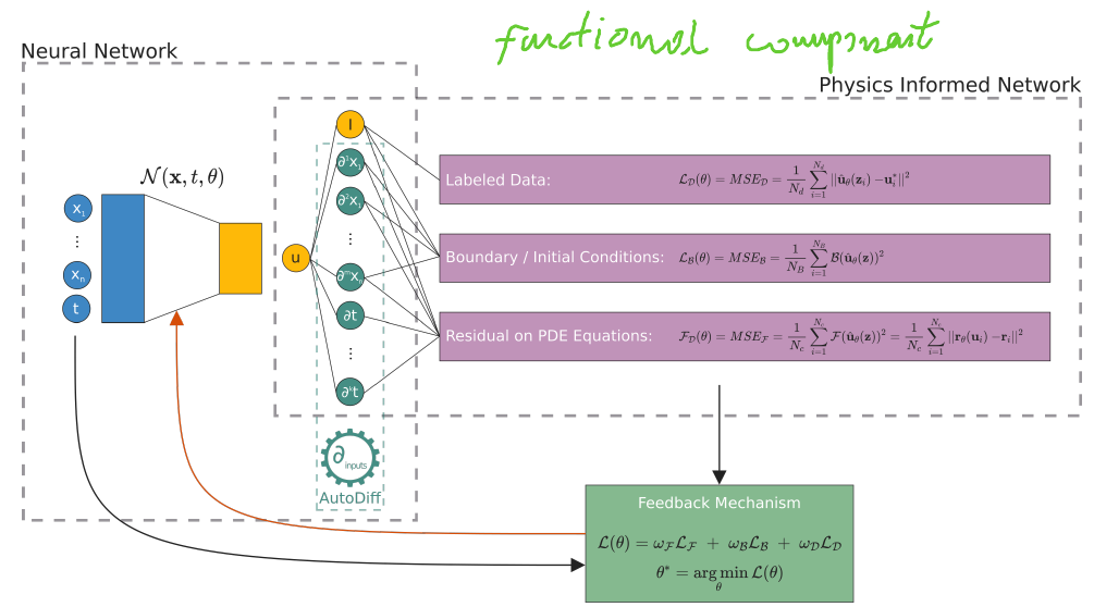 Image taken from Scientific Machine Learning through
Physics-Informed Neural Networks: Where
we are and What’s next by Cuomo, Salvatore and Di Cola, Vincenzo Schiano and Giampaolo, Fabio and Rozza, Gianluigi and Raissi, Maizar and Piccialli, Francesco, 2022.
Image taken from Scientific Machine Learning through
Physics-Informed Neural Networks: Where
we are and What’s next by Cuomo, Salvatore and Di Cola, Vincenzo Schiano and Giampaolo, Fabio and Rozza, Gianluigi and Raissi, Maizar and Piccialli, Francesco, 2022.
Here, we will solve the Heat equation $U_t=0.1U_{xx}$ with Dirichlet boundary conditions, homogeneous $U(0,t)=0$ and non-homogeneous $U(1,t)=sin(2t)$, together with the initial condition $U(x,0)=\sqrt{x}$. Non-homogeneous solutions can cause difficulties, i.e. it is often not straightforward to obtain stable convergence and model overfits easily. The problem can be overcome by applying bespoke NN architecture and/or Fourier Features. The analytical solution was obtained through Mathematica in the form of the first two terms of expansion of the solution and is plotted below. For the PINN residual term, we have 200x100 = 20000 points from which we will sample points, namely collocation points inside the domain, $\Omega$. Fourier Features are explaind in another blog post
import matplotlib.pyplot as plt
import torch
import scipy
from scipy.integrate import solve_ivp
from torch import nn
from torch import Tensor
import torch.autograd as autograd
from torch.optim import Adam, LBFGS
import numpy as np
#!pip install torchviz
from torchviz import make_dot

#!pip install jupyterthemes
from jupyterthemes import jtplot
jtplot.style(theme="grade3", context="notebook", ticks=True, grid=True)

print("CUDA available: ", torch.cuda.is_available())
device = torch.device("cuda:0" if torch.cuda.is_available() else "cpu")
print("PyTorch version: ", torch.__version__ )

def analytical_sol(x,t,y):
    x_plot =x.squeeze(1)
    t_plot =t.squeeze(1)
    X,T= torch.meshgrid(x_plot,t_plot)
    F_xt = y
    fig = plt.figure(figsize=(25,12))
    fig.suptitle('Analytical Solution of the Heat Equation', fontsize=30)

    ax1 = fig.add_subplot(121, projection='3d')
    ax2 = fig.add_subplot(122)

    ax1.plot_surface(T.numpy(), X.numpy(), F_xt.numpy(),cmap="twilight")
    ax1.set_title('U(x,t)')
    ax1.set_xlabel('t')
    ax1.set_ylabel('x')

    cp = ax2.contourf(T,X, F_xt,20,cmap="twilight")
    fig.colorbar(cp) # Add a colorbar to a plot
    ax2.set_title('U(x,t)')
    ax2.set_xlabel('t')
    ax2.set_ylabel('x')
    plt.show()

def approx_sol(x,t,y):
    X,T= x,t
    F_xt = y
    fig = plt.figure(figsize=(25,15))
    fig.suptitle('NN Approximated Solution of the Heat Equation', fontsize=30)
    ax1 = fig.add_subplot(121, projection='3d')
    ax2 = fig.add_subplot(122)

    ax1.plot_surface(T.numpy(), X.numpy(), F_xt.numpy(),cmap="twilight")
    ax1.set_title('U(x,t)')
    ax1.set_xlabel('t')
    ax1.set_ylabel('x')

    cp = ax2.contourf(T,X, F_xt,20,cmap="twilight")
    fig.colorbar(cp) # Add a colorbar to a plot
    ax2.set_title('U(x,t)')
    ax2.set_xlabel('t')
    ax2.set_ylabel('x')
    plt.show()

# We will approximate the heat equation on the box [0, 1]x[0, 1]:
x_min=0.
x_max=1.
t_min=0.
t_max=1.
#Collocation discretisation of the box, i.e. for the residual term
total_points_x=200
total_points_t=100

#Create mesh
x=torch.linspace(x_min,x_max,total_points_x).view(-1,1)
t=torch.linspace(t_min,t_max,total_points_t).view(-1,1)
# Create the mesh
X,T=torch.meshgrid(x.squeeze(1),t.squeeze(1))#[200,100]
print(x.shape)#[200,1]
print(t.shape)#[100,1]
print(X.shape)#[200,100]
print(T.shape)#[200,100]

x_min_tens = torch.Tensor([x_min])
x_max_tens = torch.Tensor([x_max])
#To get analytical solution obtained via MATHEMATICA
f_real = lambda x, t:  (1. - 1.*x)*torch.sin(2*t) +( 1.12734*torch.exp(-0.98696*t) - 0.252637*torch.cos(2.*t) - 0.511949*torch.sin(2.*t) )* torch.sin(torch.pi*x)+\
                        ( -0.112278*torch.exp(-3.94784*t) - 0.128324*torch.cos(2.*t) - 0.0650094*torch.sin(2.*t) )* torch.sin(2*torch.pi*x)
# Evaluate real solution on the box domain
U_real=f_real(X,T)
analytical_sol(x,t,U_real) #f_real was defined previously(function)

Since we approximate NN solution on $[0,1]x[0,1]=100x200$ for space and time , respectively, it is necessary to flatten our domain $\Omega$. All input vectors are two-dimensional for space and time. The output is one-dimensional, which later, after reshaping, will result in an approximated solution. For later error estimations, let us prepare the test vector and analytical solution $U$. To do so, we have to flatten input field into a two-dimensional vector $\{x_{i}, t_{i}\}_{i=1}^{20000}$ and one-dimensional output vector $\{U_{test}^{i}\}_{i=1}^{20000}$. Similar setup will be applied for the initial (IC) and boundary conditions (BC).
#Prepare testing data
# Transform the mesh into a 2-column vector
x_test=torch.hstack((X.transpose(1,0).flatten()[:,None],T.transpose(1,0).flatten()[:,None]))#[200x100 -> 20000,2]
U_test=U_real.transpose(1,0).flatten()[:,None] #[200x100 -> 20000,1] # Colum major Flatten (so we transpose it)
Now it is time to set up vectors on which NN will approximate the desired solution. The initial data at $t=0$ are from 18 points sampled from 100-points time vector, so we obtain 2-column vector $\{U_0^i, x_0^i\}_{i=1}^{18}$.
The boundaries at $x=0$ and $x=1$ consist of 150 points sampled from a 200-points spatial vector. In this way, we obtain the 2-column vector $\{U_b^i, t_0^i\}_{i=1}^{150}$.
Next, we stack IC and BCs vertically into two vectors of the length of 168 points for inputs X_train_boundaries and solution on boundaries U_train_boundaries.
# Domain bounds
lb=x_test[0] #first value of the mesh
ub=x_test[-1] #last value of the mesh

# Transform the mesh into a 2-column vector
#Left Edge: U(x,0)=sqrt(x)->xmin=<x=<xmax; t=0
left_X=torch.hstack((X[:,0][:,None],T[:,0][:,None])) #[200,2]
left_U=torch.sqrt(left_X[:,0]).unsqueeze(1) #[200,1]

#Boundary Conditions
#Bottom Edge: U(x_min=0,t) = sin(2x); tmin=<t=<max
bottom_X=torch.hstack([X[0,:][:,None],T[0,:][:,None]]) #[100,2]
bottom_U= torch.sin(2.*(bottom_X[:,1][:,None]))#[100,1]

#Top Edge: U(x_max=1,t) = 0 ; 0=<t=<1
top_X=torch.hstack((X[-1,:][:,None],T[-1,:][:,None])) #[100,2]
top_U=torch.zeros(top_X.shape[0],1) #[100,1]

N_IC=20
idx=np.random.choice(left_X.shape[0],N_IC,replace=False)
X_IC=left_X[idx,:] #[15,2]
U_IC=left_U[idx,:] #[15,1]

#Stack all boundaries vertically
X_BC=torch.vstack([bottom_X,top_X]) #[150,2]
U_BC=torch.vstack([bottom_U,top_U]) #[150,1]

N_BC=200
idx=np.random.choice(X_BC.shape[0],N_BC,replace=False)
X_BC=X_BC[idx,:] #[100,2]
U_BC=U_BC[idx,:] #[100,1]

#Stack all boundaries vertically
X_train_boundaries=torch.vstack([X_IC, X_BC]) #[185,2]
U_train_boundaries=torch.vstack([U_IC, U_BC]) #[185,1]
For the residual term, we have 200x100 = 20000 points from which we sample 10000 points. That is why the solution domain is on $U(x,t)$ are $\{ x_c^i, t_c^i \}_{i=1}^{1000}$. Next, we stack the collocation points inside the domain, $\Omega$, with those for BCs. This way, we have all the necessary arrays and vectors prepared for the training.
#Collocation Points to evaluate PDE residual
#Choose(Nf) points(Latin hypercube)
N_residual=10000
from pyDOE import lhs
X_train_residual=lb+(ub-lb)*lhs(2,N_residual)#[1000,2] # 2 as the inputs are x and t
X_train_total=torch.vstack((X_train_residual,X_train_boundaries))#[10000,2] and [100,] -> [10100,2] Add the training points to the collocation points

torch.manual_seed(123)
#Store tensors to GPU
X_train_boundaries=X_train_boundaries.float().to(device)#Training Points (BC)
U_train_boundaries=U_train_boundaries.float().to(device)#Training Points (BC)
X_train_total=X_train_total.float().to(device)#Collocation Points
U_hat = torch.zeros(X_train_total.shape[0],1).to(device)#[10100,1]; needed to loss function
X_train_residual.shape
We will apply wide, shallow NN architecture with additional skip connections to overcome the vanishing gradient problem. In addition, it is usually that the deeper NN, the more learning goes towards low-frequency features. Thus, there are applied so-called Fourier Features that prevent the omission of high-frequency functions. The used here mapping is $\gamma(x)=[cos(B\,x), sin(B\,x)]^T$ with $B$ drawn from normal distribution. tune_beta is the aggregating gradient accumulator stabilising training by smoothing irregularities and facilitating gradients' flow. The NN's architecture is depicted here .
class DenseResNet(nn.Module):

    def __init__(self, dim_in, dim_out, num_resnet_blocks,
                 num_layers_per_block, num_neurons, activation,
                 fourier_features, m_freqs, sigma, tune_beta):
        super(DenseResNet, self).__init__()

        self.num_resnet_blocks = num_resnet_blocks
        self.num_layers_per_block = num_layers_per_block
        self.fourier_features = fourier_features
        self.activation = activation
        self.tune_beta = tune_beta

        if tune_beta:
            self.beta0 = nn.Parameter(torch.ones(1, 1)).to(device)
            self.beta = nn.Parameter(torch.ones(self.num_resnet_blocks, self.num_layers_per_block)).to(device)

        else:
            self.beta0 = torch.ones(1, 1).to(device)
            self.beta = torch.ones(self.num_resnet_blocks, self.num_layers_per_block).to(device)


        self.first1 = nn.Linear(dim_in, num_neurons)
        # nn.init.xavier_uniform_(self.first1.weight.data)
        # nn.init.zeros_(self.first1.bias.data)
        self.first2 = nn.Linear(dim_in, num_neurons)
        # nn.init.xavier_uniform_(self.first2.weight.data)
        # nn.init.zeros_(self.first2.bias.data)
        self.first3 = nn.Linear(dim_in, num_neurons)
        # nn.init.xavier_uniform_(self.first3.weight.data)
        # nn.init.zeros_(self.first3.bias.data)
        self.first4 = nn.Linear(dim_in, num_neurons)
        # nn.init.xavier_uniform_(self.first4.weight.data)
        # nn.init.zeros_(self.first4.bias.data)
        self.first5 = nn.Linear(dim_in, num_neurons)
        # nn.init.xavier_uniform_(self.first5.weight.data)
        # nn.init.zeros_(self.first5.bias.data)

        self.resblocks = nn.ModuleList([
            nn.ModuleList([nn.Linear(num_neurons, num_neurons)
                for _ in range(num_layers_per_block)])
            for _ in range(num_resnet_blocks)])

        self.last = nn.Linear(num_neurons, dim_out)

        if fourier_features:
            self.first1 = nn.Linear(2*m_freqs, num_neurons)
            self.first2 = nn.Linear(2*m_freqs, num_neurons)
            self.first3 = nn.Linear(2*m_freqs, num_neurons)
            self.first4 = nn.Linear(2*m_freqs, num_neurons)
            self.first5 = nn.Linear(2*m_freqs, num_neurons)
            self.B = nn.Parameter(sigma*torch.randn(dim_in, m_freqs).to(device)) # to converts inputs to m_freqs

    def forward(self, x):
        if self.fourier_features:
            cosx = torch.cos(torch.matmul(x, self.B)).to(device)
            sinx = torch.sin(torch.matmul(x, self.B)).to(device)
            x = torch.cat((cosx, sinx), dim=1)
            x1 = self.activation(self.beta0*self.first1(x))
            x2 = self.activation(self.beta0*self.first2(x))
            x3 = self.activation(self.beta0*self.first3(x))
            x4 = self.activation(self.beta0*self.first4(x))
            x5 = self.activation(self.beta0*self.first5(x))
            id1 = x1
            id2 = x2
            id3 = x3
            id4 = x4
            id5 = x5

        else:
            x1 = self.activation(self.beta0*self.first1(x))
            x2 = self.activation(self.beta0*self.first2(x))
            x3 = self.activation(self.beta0*self.first3(x))
            x4 = self.activation(self.beta0*self.first4(x))
            x5 = self.activation(self.beta0*self.first5(x))
            id1 = x1
            id2 = x2
            id3 = x3
            id4 = x4
            id5 = x5

        for i in range(self.num_resnet_blocks):
            z1 = self.activation(self.beta[i][0]*self.resblocks[i][0](x1))
            z2 = self.activation(self.beta[i][0]*self.resblocks[i][0](x2))
            z3 = self.activation(self.beta[i][0]*self.resblocks[i][0](x3))
            z4 = self.activation(self.beta[i][0]*self.resblocks[i][0](x4))
            z5 = self.activation(self.beta[i][0]*self.resblocks[i][0](x5))

            for j in range(1, self.num_layers_per_block):
                z11 = self.activation(self.beta[i][j]*self.resblocks[i][j](z1))
                z22 = self.activation(self.beta[i][j]*self.resblocks[i][j](z2))
                z33 = self.activation(self.beta[i][j]*self.resblocks[i][j](z3))
                z44 = self.activation(self.beta[i][j]*self.resblocks[i][j](z4))
                z55 = self.activation(self.beta[i][j]*self.resblocks[i][j](z5))
                z11 = z11 + id1
                z22 = z22 + id2
                z33 = z33 + id3
                z44 = z44 + id4
                z55 = z55 + id5

                for j in range(1, self.num_layers_per_block):
                    z111 = self.activation(self.beta[i][j]*self.resblocks[i][j](z11))
                    z222 = self.activation(self.beta[i][j]*self.resblocks[i][j](z22))
                    z333 = self.activation(self.beta[i][j]*self.resblocks[i][j](z33))
                    z444 = self.activation(self.beta[i][j]*self.resblocks[i][j](z44))
                    z555 = self.activation(self.beta[i][j]*self.resblocks[i][j](z55))

                x =  z111 + z222 + z333 + z444 +z555

        out = self.last(x)

        return out

Fourier_dense_net1 = DenseResNet(dim_in=2, dim_out=1, num_resnet_blocks=3,
                        num_layers_per_block=3, num_neurons=25, activation=nn.LeakyReLU(0.65),
                        fourier_features=True, m_freqs=30, sigma=8, tune_beta=True)

PINN = Fourier_dense_net1.to(device)
x = torch.randn(2,2).to(device).requires_grad_(True)
y = PINN(x)
#make_dot(y, params=dict(list(PINN.named_parameters()))).render("Residual_net", format="png")
make_dot(y, params=dict(list(PINN.named_parameters()))).render("Residual_net_svg", format="svg")
The architecture of NN is as follow
 or in details
For the training loop, the ADAM is used, but in the last part, LFBGS tries to find the minimum of the objective function. LFBGS is the second-order optimizer that uses Hessian approximations.
X_test=x_test.float().to(device) # the input dataset (complete)
U_test=U_test.float().to(device) # the real solution

lr = 5e-4
optimizer = torch.optim.Adam(PINN.parameters(),lr=lr)#,amsgrad=True, weight_decay=1e-4)#, eps=1e-8)
optimizer_LBFGS = LBFGS(PINN.parameters(), history_size=250, max_iter=5000, line_search_fn="strong_wolfe")
loss_function = nn.MSELoss(reduction ='mean')
loss_evolution = []
iter = 0
steps = 3000
test_loss = torch.tensor([np.Inf]).to(device)

def train():
    x_BC= PINN(X_train_boundaries)
    loss_BC=loss_function(x_BC, U_train_boundaries)
    g=X_train_total.clone()
    g.requires_grad=True #Enable differentiation
    U=PINN(g)
    U_x_t = autograd.grad(U,g,torch.ones([g.shape[0], 1]).to(device), retain_graph=True, create_graph=True)[0] #first derivative
    U_xx_tt = autograd.grad(U_x_t,g,torch.ones(g.shape).to(device), create_graph=True)[0] #second derivative
    U_t=U_x_t[:,[1]]    # we select the 2nd element for t (the first one is x) (Remember the input X=[x,t])
    U_xx=U_xx_tt[:,[0]] # we select the 1st element for x (the second one is t) (Remember the input X=[x,t])
    U=U_t - 0.1*U_xx    # updated approximation
    loss_PDE = loss_function(U,U_hat)#U_hat=0 if you putt the equation on the LHS and leave 0 on the RHS
    loss = loss_BC + loss_PDE
    return loss

LOSSES = []
TEST_LOSSES = []
ITERACJE = []
U_anim = np.zeros((total_points_x,total_points_t, steps))

for i in range(steps):
    optimizer.zero_grad()
    loss = train()

    loss.backward()
    optimizer.step()

    if test_loss < 0.00085:
        def closure():
            optimizer_LBFGS.zero_grad()
            loss = train()
            loss.backward()
            return loss
        optimizer_LBFGS.step(closure)
        loss = closure()

    U_anim[:,:,i]=PINN(X_test).reshape(shape=[total_points_t,total_points_x]).transpose(1,0).detach().cpu()
    iter += 1
    if i%(steps/100)==0:

        with torch.no_grad():
            test_loss = loss_function(PINN(X_test),U_test)
            LOSSES.append(loss.detach().cpu().numpy())
            TEST_LOSSES.append(test_loss.detach().cpu().numpy())
        ITERACJE.append(iter+1)
        print(iter+1,': ', loss.detach().cpu().numpy(),'---',test_loss.detach().cpu().numpy())
fig, (ax1, ax2) = plt.subplots(2,1, figsize=(20,15))
fig.suptitle('Historical Losses', fontsize=30)
ax1.semilogy(ITERACJE[1:], LOSSES[1:], c='deeppink',linewidth=2.8, label='Train loss')
ax1.set_ylabel('Loss')
ax1.set_xlabel('Iterations')
ax1.legend()

ax2.semilogy(ITERACJE[1:], TEST_LOSSES[1:],c='dodgerblue',linewidth=2.8, label='Test loss')
ax2.set_ylabel('Test Loss')
ax2.set_xlabel('Iterations')
ax2.legend()
plt.show()

To obtain better results, it is advesible to extend traing to LFBGS part, however the usage of this optimisation algorithm is very time-consuming.
U1=PINN(X_test)
x1=X_test[:,0]
t1=X_test[:,1]

arr_x1=x1.reshape(shape=[total_points_t,total_points_x]).transpose(1,0).detach().cpu()
arr_T1=t1.reshape(shape=[total_points_t,total_points_x]).transpose(1,0).detach().cpu()
arr_U1=U1.reshape(shape=[total_points_t,total_points_x]).transpose(1,0).detach().cpu()
arr_U_test=U_test.reshape(shape=[total_points_t,total_points_x]).transpose(1,0).detach().cpu()

approx_sol(arr_x1,arr_T1,arr_U1)

It is effective to visualise the learning process. There are two animations below for 3-D and contour plots.
The results of PINN is not as accurate as those obtained by numerical methods (finite difference or Method of Lines), but it shows that this novel approach works and is very promising for further research.
ANIMATIONS
If you are interested in creating animations read the further part of the post.
Contour plot
#!conda install -c conda-forge ffmpeg
from mpl_toolkits.mplot3d import Axes3D
import matplotlib.animation as animation
#import networkx as nx
from matplotlib.animation import FuncAnimation, PillowWriter, MovieWriter
from IPython.display import HTML

#Contour plt
fps = 20 # frame per sec
frn = 1# frame number of the animation; the lower value the more frames

xarray = []
for i in range(steps):
    if i%frn == 0:
        xarray.append(U_anim[:,:,i])
carray = np.einsum('kil->ilk', np.array(xarray))

fig, ax = plt.subplots(figsize=(20,18))
fig.suptitle('Solution of Approximated Heat Equation', fontsize=30)
def animate(i):
    ax.clear()
    ax.contourf(T.numpy(), X.numpy(),carray[:,:,i], 30, cmap="twilight")
ani_2 = animation.FuncAnimation(fig, animate, carray.shape[2], interval=500, repeat=False)
fn = 'plot_contour_animation_funcanimation'
#ani_2.save(fn+'.gif',writer='imagemagick',fps=fps)
ani_2.save(fn+'.mp4',writer='ffmpeg',fps=fps)
To deploy plot in notebook
import matplotlib
matplotlib.rcParams['animation.embed_limit'] = 2**128
plt.rcParams['animation.html'] = 'html5'
ani_2
3-D surface plot
This is how to creat top page surface animation.
fps = 20 # frame per sec
frn = 10# frame number of the animation; the lower value the more frames

xarray = []
for i in range(steps):
    if i%frn == 0:
        xarray.append(U_anim[:,:,i])
carray = np.einsum('kil->ilk', np.array(xarray))


def update_plot(frame_number, zarray, plot):
    plot[0].remove()
    plot[0] = ax.plot_surface(T.numpy(), X.numpy(), carray[:,:,frame_number], cmap="twilight")


fig = plt.figure(figsize=(20,18))
fig.suptitle('Solution of Approximated Heat Equation', fontsize=30)
ax = fig.add_subplot(111, projection='3d')

plot = [ax.plot_surface(T.numpy(), X.numpy(), carray[:,:,0], color='0.75', rstride=1, cstride=1)]
ax.set_zlim(0,1.1)
ani = animation.FuncAnimation(fig, update_plot, steps//frn, fargs=(carray, plot), interval=5000/fps)

ax.set_title('$U(x,t)_{approximated}$')
ax.set_xlabel('t')
ax.set_ylabel('x')
fn = 'plot_surface_animation_funcanimation'
ani.save(fn+'.mp4',writer='ffmpeg',fps=fps)
ani.save(fn+'.gif',writer='imagemagick',fps=fps)
Physics-Informed Neural Networks (PINNs) have shown promise in solving Partial Differential Equations (PDEs) by incorporating physical laws into the learning process. However, they face challenges like lack of invariance to the mesh, which can affect their accuracy and generalization. On the other hand, the Neural Operator approach, inspired by the principles of Neural Networks and Operators, offers a way to learn mappings between function spaces, inherently providing mesh invariance. This feature of Neural Operators can significantly enhance the model's capability to generalize across different meshes, thus potentially overcoming a key limitation faced by PINNs in solving PDEs. For a deeper understanding, refer to the seminal paper on Neural Operators.
In the next post, I will look at the inverse problem.
