Convolution Atlas: from discrete sums to Legendre geometry
Convolution becomes easier to follow when each term in the formula has a visible counterpart. Convolution Atlas connects the samples, their products and the output, then follows coefficient matching into the geometry of Legendre polynomials.
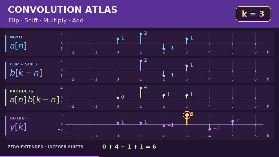
Start with a finite sum
In the discrete convolution lesson, choose an example or edit the samples. Flip and slide the kernel, inspect a product, then watch the products add to one output value. The formula and plot colours match, so a selected term can be followed across the views.
The three views show the complete sequences, the flip–slide–sum construction, and the addition of shifted kernels. This lesson uses finite point samples, with zero values away from their sample positions.
From coefficient matching to geometry
The Joukowski–Legendre lesson follows a different use of convolution: multiplying two generating series and collecting terms of the same degree. A lattice shows which pairs contribute, while the complex-plane diagrams show the corresponding Laurent powers.
Move the angle and radius to connect the circle, its Joukowski image and the Legendre mode. The degree selected in the generating series and the Fourier frequency of a Laurent term remain distinct throughout the explanation.
Why the real-line bound is one
In real-line stability, the circle has radius one. A point and its reciprocal are complex conjugates; their midpoint is the real input. Linked diagrams then show the Legendre value as a weighted mean of unit phases. Positive weights summing to one keep that mean inside the unit disk, and the endpoint normalization attains one.
The lesson includes the angular integral estimate used later in the thesis. The displayed argument supplies the bound; the moving diagrams and numerical readouts help explain it.
Choose your starting point
The atlas is growing one lesson at a time. These three linked lessons are available now, with mathematical notation rendered through MathJax.