SVD
![]()
SVD and Dimensionality Reduction
Given $X\in \mathbb{R}^{s\times n}$, consider the low rank approximation problem $$ \underset{R}{\min }\, \| X-R\| _{\text{Fro}}^2\,\,\,subject\,\,to\,\, rank(R)=k$$ where $\| A\| _{\text{Fro}}\text{:=}\,\sum _{i=1}^s \sum _{j=1}^n a _{\text{ij}}^2$, the entrywise squared $\ell_2$ norm.
To understand the PCA, it is good to delve into SVD matrix decomposition, the kernel of data compression, recommender systems, linear autoencoders and umpteen other machine-learning applications. SVD is the generalisation of Fourier transformation to more complex systems. In other words, SVD is a matrix factorisation that generalises the concept of eigendecopmpositions of square matrices. Namely, it can be shown that every real (and complex) matrix $X\in \mathbb{R^{s\times n}}$ can be factorised into three matrices $U\in \mathbb{R^{s\times s}}$, $\Sigma \in \mathbb{R^{s \times n}}$ and $V \in \mathbb{R^{n \times n}}$ through
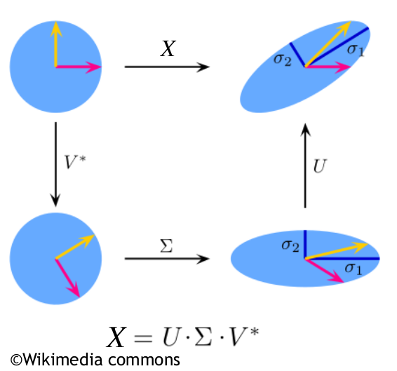
$$X = U \Sigma V^*\,\,\,\,(2.10)$$
Here both $U$ and $V$ are unitary matrices of eigenvectors whose columns are called left and right singular vectors of $X$. For the real matrices $X = U \Sigma V^T=\sigma_1U_1V^T_1+\sigma_2 U_2 V^T_1 +...+\sigma_n U_n V^T_n$. The The matrix $\Sigma$ is a diagonal matrix of decreasing eigenvalues of the form:
-
for $s>n$ $$\left( \begin{array}{cccc} \sigma _1 & 0 & \ldots & 0 \\ 0 & \sigma _2 & \ldots & 0 \\ 0 & 0 & \ddots & 0 \\ 0 & 0 & \ldots & \sigma _n \\ 0 & 0 & \ldots & 0 \\ \vdots & \vdots & \ddots & 0 \\ 0 & 0 & \ldots & 0 \\ \end{array} \right)$$
-
for $s<n$
$$\left(
\begin{array}{ccccccc}
\sigma _1 & 0 & \cdots & 0 & 0 & \cdots & 0 \\
0 & \sigma _2 & \cdots & 0 & 0 & \cdots & 0 \\
0 & 0 & \ddots & 0 & 0 & \cdots & 0 \\
0 & 0 & \ldots & \sigma _s & 0 & \ldots & 0 \\
\end{array}
\right)$$
SVD means that every matrix can be expressed by rotation -> scaling -> another rotation that is illustrated below
 ** Make Wiki dontation!!! **
- for $s=n$ there is a symmetric singular matrix. The entrie $\{\sigma_j\}_{j=1}^{min (s,n)}$ are called singular values of $X$, and are all-nonnegative, i.e. ${\sigma_j \geq 0 \,\,\forall j\in\{1,...,min(s,n)\}}$. Notice that SVD of $X$ allows us to easily compute the Frobienius norm, $\| \Sigma \| _{\text{Fro}}^2=\sqrt{\sum _{i=1}^s \sum _{j=1}^n \left| x_{\text{ij}}\right| {}^2}$, of that matrix since the Frobenius norm is equivalent to the Euclidian (EU) norm of the vector of singular values, which we see from $$\| \Sigma \| _{\text{Fro}}^2=\langle X,X\rangle =\left\langle \text{U$\Sigma $V}^T,\text{U$\Sigma $V}^T\right\rangle =\left\langle \text{$\Sigma $V}^T,U^T \text{U$\Sigma $V}^T\right\rangle =\left\langle \Sigma ,\text{V$\Sigma $} V^T\right\rangle =\langle \Sigma ,\Sigma \rangle =\| \Sigma \| _{\text{Fro}}^2=\sum _{j=1}^{\min (S,n)} \sigma _j^2$$
SVD can be used for the ** best matrix approximation ** of matrix $X$ in terms of the Frobenius norm. For instance, images can be compressed, or in the recommender system, we can approximate recommendations through lower-rank matrices. Suppose we define a new matrix $U_k \in \mathbb{R}^{s \times k}$ as the first $k$ columns of $U$. Then we observe that our k-rank approximated matrix $X_k$ $$X_k=X U_k U_k^T=U_k U_k \text{U$\Sigma $V}^T=U_k \left(I_{k\times k} \,\,\,0_{k\times (s-k)}\right)\text{$\Sigma $V}^T =\text{U$\Sigma $}_k V^T=X_k$$ where $\Sigma _k\in \mathbb{R}^{s\times n}$ as
$$\Sigma _k=\left( \begin{array}{ccccccc} \sigma _1 & 0 & \ldots & 0 & 0 & \cdots & 0 \\ 0 & \sigma _2 & \ldots & 0 & 0 & \cdots & 0 \\ 0 & 0 & \ddots & 0 & \vdots & \ddots & \vdots \\ 0 & 0 & \ldots & \sigma _k & 0 & \cdots & 0 \\ 0 & 0 & \ldots & 0 & 0 & \cdots & 0 \\ \vdots & \vdots & \ddots & 0 & \vdots & \ddots & \vdots \\ 0 & 0 & \ldots & 0 & 0 & \ldots & 0 \\ \end{array} \right)$$
Therefore to reconstruct apprximated matrix based on the most relevant information deployed in subspaces, we can
$$\underset{U_k,U_k^T}{\min }\left\| X-X \underbrace{U_k^T U_k}_Z \right\|_{\text{Fro}}^2=\underset{\left\{\sigma_j\right\}_{j=1}^{k < \min (s,n)}}{\min }\left\| X-\underbrace{\text{U$\Sigma $}_k V^T}_{R}\right\| _{\text{Fro}}^2$$
You can observe that $\underbrace{U_k^T U_k}_Z $ is positive semi-definite Hessian in the quadratic term. Hence the hard conbinatorial problem is re-written into convex optimisation task. In more details, having gram matrix $S=X^T X$, the $Z$ is the projection $\Longleftrightarrow$ $\underset{Z\in \mathbb{S}^n}{\max }\,\,\, tr(SZ)$ subject to $rank(Z)=k$, there is non-nonconvex constraint set
$$C=\left\{ Z\,\in \mathbb{S}^n\,:\,\lambda_i(Z)\,\in\, \left\{0,1 \right\},\,i=1,...,n\,\,\,, tr(Z)=k \right\}$$
where $\lambda_i(Z),\,\,,i=1,...,s$ are eigenvalues of $Z$ and $\mathbb{S}$ is n-dimensional space.
The solution of the above formulation is
$$Z=V_k V_k^T$$
where $V_k$ gives $k$-first columns of $V$.
Now, by Fan (1949), let's relax the constraint set to
$$F=\left\{ Z\,\in \mathbb{S}^n\,:\,\lambda_i(Z)\,\in\, [0,1 ],\,i=1,...,n\,\,\,, tr(Z)=k \right\}=\left\{ Z\,\in \mathbb{S}^n\,:\,\,0 \preceq I \preceq Z\,\,, tr(Z)=k \right\}$$
Namely, $\underset{Z\in \mathbb{S}^n}{\max }\,\,\, tr(SZ)$ is convex problem.
Regarding error, the Eckart-Young_Mirsky theorem states that for any data matrix $X$ and any matrix $\hat{X}$ with $rank(\hat{X})=k$, we have the ** error of approximation ** as follows
$$\left\| X-\hat{X}\right\| _{\text{Fro}}^2\geq \left\| X-X_k\right\| _{\text{Fro}}^2=\left\| X-X U_k U_k^T\right\| _{\text{Fro}}^2=\sum _{j\geq k+1}^{\min (s,n)} \sigma _j^2$$
Thus by computing SVD of matrix $X$ and taking k-first columns of $U$ we obtain the best k-rank matrix approximation in terms of the Frobenius norm. The last term in the above formula is the sum of sinular values beyond $X_k$.
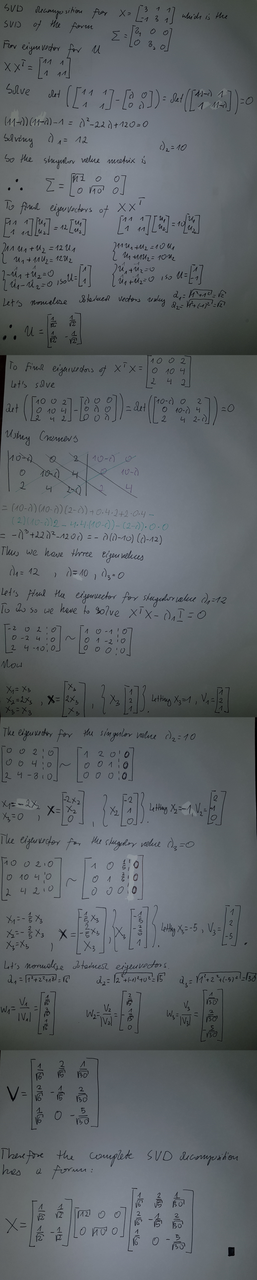
If we want to perform SVD of matrix $X$ by hand, first, we have to find eigenvalues of $XX^T$ by computing the characteristic polynomial. Then we compute eigenvectors in the nullspace of $XX^T -\lambda I$, where $\lambda's$ are roots of the characteristic polynomial. We can use Gaussian elimination or Gram-Schmidt's process. There is the example here.
Let's compute approximations of the original image by setting all singular values after the given index to zero and print the ratios of the Frobenius norm of approximations to the original matrix. As you will see from the plotted pictures, the closer the ratio is to one, the better an approximation. We will work on the image as below.
import matplotlib.pyplot as plt
import numpy as np
#!pip install scikit-image
from skimage import data
image1 = data.astronaut()
print(image1.shape)
plt.imshow(image1)
plt.show()

Since it is an RGB image, we have to reshape it accordingly.
matrix = image1.reshape(-1, 1536) # -> (512, 1536)
print(matrix.shape)
The first step is to perform SVD decomposition and visualise singular values.
U, sing_vals, V_transpose = np.linalg.svd(matrix)
print('U: ', U.shape)
print('sing_vals: ', sing_vals.shape)
print('V_transpose: ', V_transpose.shape)
fig = plt.figure()
ax = fig.add_subplot(1,1,1)
ax.plot(sing_vals, lw=2, c = 'deeppink')
ax.set_yscale('log')
ax.set_xlabel('K')
ax.set_ylabel('Singular Values')

To approximate our image from SVD matrices, we form a diagonal matrix $\Sigma_k$ based on the thresholded singular values, i.e., we zero out all the singular values after the threshold. To recover the approximation matrix, we multiply matrices $X_{k}= U \Sigma_k V^T$. The approximation results are shown below. Note that the image is standardised.
# To perform PCA center the data
matrix = matrix - np.mean(matrix, axis=1).reshape(matrix.shape[0], 1)
# In practice the full standardisation is often applied
#matrix = matrix/np.std(matrix, axis=1).reshape(matrix.shape[0], 1)
def plot_approx_img(indexes, U, sing_vals, V_transpose ):
_, axs = plt.subplots(nrows=len(indexes)//2, ncols=2, figsize=(14,26))
axs = axs.flatten()
for index, ax in zip(indexes, axs):
sing_vals_thresholded = np.copy(sing_vals)
sing_vals_thresholded[index:] = 0 # zero out all the singular values after threshold
ratio = np.sum(sing_vals_thresholded**2)/np.sum(sing_vals**2) # compute the ratio
Sigma = np.zeros(matrix.shape)
#form zero-truncated matrix of singular values
Sigma[:matrix.shape[0], :matrix.shape[0]] = np.diag(sing_vals_thresholded)
matrix_approx = U@(Sigma@V_transpose) # approximated matrix
#image reshaping and clipping
image_approx = matrix_approx.reshape(image1.shape)
img = np.rint(image_approx).astype(int).clip(0, 255)
ax.imshow(img)
ax.set_title(['Threshold is '+str(index), 'Explaind in ' + str(round(ratio, 4))])
thresholds = np.array([2] + [4*2**k for k in range(7)])
plot_approx_img(thresholds, U, sing_vals, V_transpose)

An image of Eileen Collins and several low-rank approximations for k=2.4,8,16,32,64,128,256.
In context of PCA, the singular vectors are referred to as principal components, and the decomposition is known as principal component analysis. Note that the singular vector $u_1$ corresponds to the largest singular value $\sigma_1$. That is why $u_1$ is the vector picturing feature of the largest variance. The only key difference compared to the SVD is the centring of the data, i.e. we subtract the mean of the columns of the data matrix. For the probabilistic PCA implamantation via eigendecomposition of covariance or correlation matrix, look here .
SDV for Peer-to-Peer MarketPlace Recommender System
Based on the overview of Depop's website, it is evident that the platform focuses on a wide range of fashion categories, including menswear, womenswear, and popular brands, with a variety of products like tops, bottoms, coats, jackets, shoes, accessories, and jewelry. This diversity offers a rich dataset for a toy recommender system based on SVD (Singular Value Decomposition) matrix decomposition.
Implementing an SVD-based Recommender System for Depop:
-
Data Collection: Compile user interaction data with products, including purchases, likes, and views, as well as product details like category, brand, and price.
-
Matrix Creation: Construct a user-item matrix where rows represent users and columns represent items. The entries in this matrix are the user's interactions with the items (e.g., ratings or frequency of purchases).
-
Applying SVD: Perform Singular Value Decomposition on the user-item matrix. SVD decomposes the matrix into three matrices - representing the latent features of users, items, and the strength of these features. This process helps in reducing the dimensionality of the data while preserving its essential characteristics.
-
Prediction and Recommendation: Use the decomposed matrices to predict a user's preference for an item they haven't interacted with yet. Recommendations are then made based on these predicted preferences, focusing on items with the highest predicted interest for each user.
-
Incorporating Social Media Trends: Enhance the recommender system by integrating social media trends, which can be used as additional data points for understanding user preferences and emerging fashion trends.
-
Continuous Learning: Continuously update the model with new user interactions and product listings to keep the recommendations relevant and timely.
Such a system would help Depop in personalizing the shopping experience for its users, leading to increased user engagement, customer satisfaction, and potentially higher sales.
The interaction matrix is generated randomly, where 0 represents no interaction, and 1 to 5 can represent different levels of interaction (like views, likes, ratings).
import pandas as pd
import numpy as np
# Parameters
num_users = 50
num_items = 20 # Reduced for illustration
# Sample items based on Depop categories and brands
items = ['Vintage_Dress', 'Adidas_Sneakers', 'Levi_Jeans', 'Supreme_Tshirt',
'Nike_Jacket', 'Boho_Skirt', 'VictoriaSecret_Bra', 'Zara_Top',
'DrMartens_Boots', 'Puffer_Jacket', 'Cyberpink_Shorts', 'Patagonia_Backpack',
'Retro_Sunglasses', 'Designer_Handbag', 'Graphic_Tee', 'Streetwear_Hoodie',
'Bohemian_Scarf', 'Casual_Sneakers', 'Formal_Blouse', 'Festival_Accessories']
# Create a random user-item interaction matrix
interaction_matrix = np.random.choice([0, 1, 2, 3, 4, 5],
size=(num_users, num_items),
p=[0.8, 0.05, 0.05, 0.03, 0.03, 0.04])
# Convert to DataFrame
df = pd.DataFrame(interaction_matrix,
index=[f'VintageLover_{i}' if i%4 == 0 else
f'VictoriaSecretFan_{i}' if i%4 == 1 else
f'CyberPinkEnthusiast_{i}' if i%4 == 2 else
f'TrendyUser_{i}' for i in range(num_users)],
columns=items)
# Display the first few rows
df.head()
In collaborative filtering, recommendations are made based on the interactions or behaviors of other users. The SVD method identifies patterns and relationships within the user-item interaction data to make predictions. It doesn't rely on the content of the items themselves (as in content-based filtering) but rather on how users have interacted with those items. This approach is particularly powerful in uncovering latent factors that represent underlying user preferences and item characteristics.
import pandas as pd
matrix = df.values # Converts the DataFrame into a NumPy matrix for numerical operations.
# Center the data
matrix_centered = matrix - np.mean(matrix, axis=1).reshape(-1, 1) # Centers the data by subtracting the mean of each user's ratings.
# Apply SVD
U, sing_vals, V_transpose = np.linalg.svd(matrix_centered, full_matrices=False) # Decomposes the matrix using SVD.
def make_recommendations_with_scores(df):
matrix = df.values # Converts the DataFrame into a NumPy matrix for numerical operations.
print('matrix: ', matrix.shape)
# Center the data
matrix_centered = matrix - np.mean(matrix, axis=1).reshape(-1, 1)
print('matrix_centered: ', matrix_centered.shape)
# Apply SVD
U, sing_vals, V_transpose = np.linalg.svd(matrix_centered, full_matrices=False)
print('U: ', U.shape)
print('sing_vals: ', sing_vals.shape)
print('V_transpose: ', V_transpose.shape)
# Use only the columns of U corresponding to non-zero singular values
reduced_U = U[:, :len(sing_vals)]
# Compute all user preferences
all_user_preferences = np.dot(reduced_U, np.diag(sing_vals))
print('all_user_preferences: ', all_user_preferences.shape)
# Compute all item scores
all_item_scores = np.dot(all_user_preferences, V_transpose)
print('all_item_scores: ', all_item_scores.shape)
return all_item_scores
recommended_items_with_scores = make_recommendations_with_scores(df)
print(recommended_items_with_scores.shape)
import pandas as pd
import numpy as np
import plotly.graph_objs as go
from IPython.display import HTML
# Create a Plotly heatmap to visualize the scores matrix
def plot_scores(matryca):
heatmap = go.Heatmap(
z=matryca,
x=df.columns, # Assuming the columns of the DataFrame are the item names
y=['User {}'.format(i) for i in range(matryca.shape[0])],
colorscale='Picnic'
)
# Create the figure and display it
fig = go.Figure(data=[heatmap])
fig.update_layout(
height=800,
title="User-Item Scores Heatmap",
xaxis_title="Items",
yaxis_title="Users"
)
#fig.show()
fig.write_html('../files/plotly/heat_svd_simple.html')
display(HTML('../files/plotly/heat_svd_simple.html'))
plot_scores(recommended_items_with_scores)
import seaborn as sns
import matplotlib.pyplot as plt
from jupyterthemes import jtplot
jtplot.style(theme="monokai", context="notebook", ticks=True, grid=True)
# Reverse the order of rows in the dataframes
df_flipped = df.iloc[::-1]
recommended_items_with_scores_flipped = recommended_items_with_scores[::-1]
fig, axs = plt.subplots(nrows=1, ncols=2, figsize=(20, 10), constrained_layout=True)
# Original Matrix Heatmap (flipped)
sns.heatmap(df_flipped, cmap="PuRd", ax=axs[0], cbar=False, yticklabels=True)
axs[0].set_title("Original User-Item Interaction Matrix")
axs[0].set_xticklabels(axs[0].get_xticklabels(), rotation=45, ha='right')
axs[0].set_yticklabels(df_flipped.index, rotation=0)
# Reconstructed Matrix Heatmap (flipped)
sns.heatmap(recommended_items_with_scores_flipped, cmap="PuRd", ax=axs[1], xticklabels=items, yticklabels=df_flipped.index)
axs[1].set_title("Reconstructed Matrix after SVD")
axs[1].set_xticklabels(axs[1].get_xticklabels(), rotation=45, ha='right')
axs[1].set_yticklabels(df_flipped.index, rotation=0)
plt.show()

In the context of the SVD applied to the user-item interaction matrix, negative values in the resulting score matrix can occur due to the centering step. When you center the data by subtracting the mean rating for each user, you're effectively normalizing their ratings around zero. Therefore, any original score below the user's average becomes negative after centering.
In the resulting score matrix after applying SVD:
- Positive values suggest that the item is predicted to be rated above the user's average.
- Negative values suggest that the item is predicted to be rated below the user's average.
These values do not necessarily represent negative interactions or dislikes; they are relative to the user's average rating. When generating recommendations, you would typically look for items with the highest scores, meaning they are the most positively deviant from the user's mean and thus of the most interest to the user according to the model.
To avoid negative values in the scores matrix, you could adjust the methodology as follows:
-
Avoid Centering: Do not subtract the mean of each user's ratings. This will ensure all original scores stay positive if they were originally positive.
-
Use Non-Negative Matrix Factorization (NMF): Instead of SVD, which can produce negative components, use NMF, which constrains the factors to be non-negative, ensuring that all predicted scores are also non-negative.
