Adversarial Attacks on Model for CIFAR-10
CIFAR-10 Classification and Adversarial Robustness
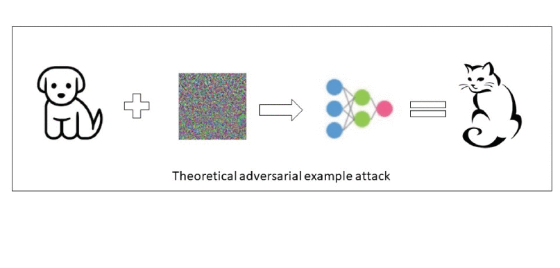
This notebook trains and evaluates an image classifier on CIFAR-10, a benchmark dataset of 60,000 colour images split into 50,000 training images and 10,000 test images. Each image belongs to one of ten classes: plane, car, bird, cat, deer, dog, frog, horse, ship, and truck. The first objective is high clean test accuracy. The second objective is to measure whether that clean accuracy survives small adversarial perturbations.
The active source notebook follows a two-stage path. First, an AirBench96-style CIFAR model is trained as a fast teacher and baseline. Second, an ImageNet-pretrained ConvNeXt-Small model is fine-tuned on CIFAR-10 using that teacher through knowledge distillation. The final checkpoint is then evaluated with ordinary test accuracy, test-time augmentation (TTA), class-wise confusion matrices, and three white-box untargeted $L_\infty$ attacks: FGSM, I-FGSM/BIM, and PGD.
Adversarial attacks are not only an academic curiosity. In practical AI work they are often used as a controlled stress test, a product feature, or the core service of an AI assurance business. Six common examples are:
- Marketing and brand-safety systems: testing whether small image edits can make visual search, ad classifiers, or brand-logo detectors miss restricted content or mislabel a product category.
- Fraud, compliance, and identity verification: checking whether document classifiers, face-matching pipelines, or transaction-risk models can be fooled by small changes that preserve the human-visible meaning.
- Military and defense AI: red-teaming object detection, reconnaissance, and sensor-fusion models so that safety-critical systems are evaluated against camouflage, spoofing, and adversarially optimized inputs before deployment.
- Political analytics and public-interest auditing: evaluating whether voter-segmentation, sentiment, or misinformation-detection models are brittle under small wording, image, or metadata changes, with the goal of detecting manipulation risk rather than enabling it.
- Medical and industrial inspection: validating whether diagnosis-support models or defect-detection systems remain stable when scans, camera images, or sensor readings contain realistic noise, compression, or acquisition artifacts.
- AI security products and model governance: offering adversarial testing, robustness certification, monitoring, and adversarial training as a service for companies that deploy high-value computer-vision or multimodal models.
This structure is deliberate. CIFAR-10 is small, so training a very large model from scratch can overfit quickly. Starting from ImageNet-pretrained ConvNeXt features gives the model a strong visual representation before CIFAR fine-tuning begins. The AirBench96 teacher adds a CIFAR-specific signal, while the adversarial section tests whether high natural accuracy should be interpreted as robustness. The answer from this notebook is no: the final model is accurate on clean CIFAR-10, but PGD still breaks it.
Data Preparation
The notebook uses a local CIFAR-10 copy and keeps download=False so repeated runs do not download the dataset again. The setup cell searches for cifar-10-batches-py, then builds a plain 32x32 tensor version of the training split to inspect the raw data. The active training and evaluation datasets are built separately afterward.
There are two active data views. The training view is stochastic and applies augmentation. The evaluation view is deterministic and is used for clean train accuracy, test accuracy, confusion matrices, TensorRT reloads, and adversarial attacks. Keeping these views separate matters because the reported metrics should measure the model on a fixed test distribution, not on randomly distorted samples.
For the ConvNeXt99 path, CIFAR-10 images are resized from 32x32 to 224x224 and normalized with ImageNet mean and standard deviation. This is not because CIFAR-10 naturally has ImageNet statistics. It is because the main classifier starts from ImageNet-pretrained ConvNeXt weights, and those weights expect the ImageNet input scale and channel normalization used during pretraining. The attack cells still define $\epsilon$ in pixel space and convert it into normalized tensor coordinates before applying perturbations.
%matplotlib inline
import copy
import os
import sys
import sysconfig
import time
from pathlib import Path
def prepend_env_path(name, paths):
existing = [path for path in os.environ.get(name, "").split(os.pathsep) if path]
new_paths = [str(path) for path in paths if Path(path).exists()]
os.environ[name] = os.pathsep.join(dict.fromkeys(new_paths + existing))
def prepend_env_flags(name, flags):
existing = os.environ.get(name, "").split()
new_flags = [str(flag) for flag in flags if flag]
os.environ[name] = " ".join(dict.fromkeys(new_flags + existing))
def configure_tensorrt_linker_paths():
conda_prefix = Path(sys.prefix)
cuda_home = Path(os.environ.get("CUDA_HOME", "/usr/local/cuda"))
link_dirs = [
conda_prefix / "lib",
cuda_home / "lib64",
cuda_home / "targets/x86_64-linux/lib",
Path("/lib/x86_64-linux-gnu"),
Path("/usr/lib/x86_64-linux-gnu"),
]
link_dirs = [path for path in link_dirs if path.exists()]
prepend_env_path("LIBRARY_PATH", link_dirs)
prepend_env_path("LD_LIBRARY_PATH", link_dirs)
prepend_env_path("CMAKE_LIBRARY_PATH", link_dirs)
linker_flags = []
for path in link_dirs:
linker_flags.extend([f"-L{path}", f"-Wl,-rpath-link,{path}"])
for path in [conda_prefix / "lib", cuda_home / "lib64"]:
if path.exists():
linker_flags.append(f"-Wl,-rpath,{path}")
prepend_env_flags("LDFLAGS", linker_flags)
sysconfig.get_config_vars()
flag_text = " ".join(linker_flags)
for key in ("LDSHARED", "BLDSHARED", "LINKCC"):
value = sysconfig.get_config_var(key)
if isinstance(value, str) and flag_text and flag_text not in value:
sysconfig._CONFIG_VARS[key] = f"{value} {flag_text}"
if not (conda_prefix / "lib" / "libaio.so").exists():
raise RuntimeError("libaio is missing. Install it with: conda install -c conda-forge libaio")
configure_tensorrt_linker_paths()
import torch
import torch.nn as nn
import torch.nn.functional as F
import torch.optim as optim
import torchvision
import torch_tensorrt
from torchvision import datasets, transforms, models
from torch.utils.data import DataLoader
############################ To depict your neural network ################################################
#!pip install torchviz
from torchviz import make_dot
from graphviz import Digraph
########################### If you want to use TensorBoard ###############################################
#from torch.utils.tensorboard import SummaryWriter
########################## To plot #######################################################################
import numpy as np
import matplotlib.pyplot as plt
from matplotlib.colors import LinearSegmentedColormap, PowerNorm
try:
from tqdm import tqdm
except ImportError:
tqdm = None
# Keep autoreload disabled: compiled modules such as pyarrow, pandas, torch, and TensorRT
# cannot be safely reloaded by IPython's superreload machinery.
%load_ext autoreload
%autoreload 0
################### to dispaly confusing matrix properly install 'jupyterthemes' ########################
#!conda install -c conda-forge jupyterthemes # - for confusion matrix
from jupyterthemes import jtplot
jtplot.style(theme="grade3", context="notebook", ticks=True, grid=True)
#########################################################################################################
NOTEBOOK_DIR = Path("/home/lucy/Documents/web10/posts")
MODELS_DIR = NOTEBOOK_DIR / "Models"
BEST_CHECKPOINT_PATH = MODELS_DIR / "checkpoint_convnext99_airbench_teacher.pt"
CHECKPOINT_PATH = BEST_CHECKPOINT_PATH
TRAIN_CHECKPOINT_PATH = CHECKPOINT_PATH
RESUME_CHECKPOINT_PATH = MODELS_DIR / "resume_convnext99_airbench_teacher.pt"
FINETUNE_RESUME_CHECKPOINT_PATH = RESUME_CHECKPOINT_PATH
TRAINING_LOG_PATH = NOTEBOOK_DIR / "training_live_output.log"
STOP_TRAINING_PATH = NOTEBOOK_DIR / "STOP_TRAINING_NOW"
CONVNEXT99_IMAGE_SIZE = 224
CONVNEXT99_BATCH_SIZE = 64
CONVNEXT99_USE_PRETRAINED = True
CONVNEXT99_VARIANT = "small"
CONVNEXT99_LINEAR_EPOCHS = 0
CONVNEXT99_FINETUNE_EPOCHS = 30
CONVNEXT99_TARGET_ACC = 0.9900
IMAGENET_MEAN = (0.485, 0.456, 0.406)
IMAGENET_STD = (0.229, 0.224, 0.225)
ACTIVE_MEAN = IMAGENET_MEAN
ACTIVE_STD = IMAGENET_STD
def make_training_run_paths(prefix="convnext99_manual"):
run_id = time.strftime("%Y%m%d_%H%M%S")
return (
MODELS_DIR / f"checkpoint_{prefix}_{run_id}.pt",
MODELS_DIR / f"resume_{prefix}_{run_id}.pt",
)
def request_training_stop(stop_path=STOP_TRAINING_PATH):
stop_path = Path(stop_path)
stop_path.write_text(f"stop requested at {time.strftime('%Y-%m-%d %H:%M:%S')}\n")
print(f"Stop requested. Training will save and stop at the next batch boundary: {stop_path}")
def clear_training_stop_request(stop_path=STOP_TRAINING_PATH):
stop_path = Path(stop_path)
if stop_path.exists():
stop_path.unlink()
print(f"Cleared stale stop request: {stop_path}")
classes = ('plane', 'car', 'bird', 'cat', 'deer', 'dog', 'frog', 'horse', 'ship', 'truck')
CIFAR_MEAN = (0.4914, 0.4822, 0.4465)
CIFAR_STD = (0.2470, 0.2435, 0.2616)
confusion_cmap = LinearSegmentedColormap.from_list(
"confusion_mint_blue_orange",
[
(0.00, "#bee5da"),
(0.10, "#bee5da"),
(0.22, "#a8d4d4"),
(0.34, "#88bfd0"),
(0.46, "#63a2ca"),
(0.62, "#8d4658"),
(0.84, "#7f3f52"),
(0.92, "#dc7040"),
(1.00, "#f6c58d"),
],
)
confusion_norm = PowerNorm(gamma=0.45, vmin=0, vmax=1000, clip=True)
print("CUDA available: ", torch.cuda.is_available())
device = torch.device("cuda:0" if torch.cuda.is_available() else "cpu")
print("PyTorch version: ", torch.__version__ )
print("Torch-TensorRT version: ", torch_tensorrt.__version__ )
The first dataset cell checks the local CIFAR-10 data and computes basic channel statistics from the original 32x32 images. This gives a sanity check on the raw dataset and confirms that the source notebook is using the local data directory rather than silently redownloading anything. The active ConvNeXt path later switches to ImageNet normalization because the main model is initialized from ImageNet-pretrained weights.
#! mkdir Data_Sets
from pathlib import Path
def resolve_cifar_root():
candidates = [
Path("./Data_Sets/Cifar10"),
Path("./posts/Data_Sets/Cifar10"),
Path("/home/lucy/Documents/web10/posts/Data_Sets/Cifar10"),
]
for path in candidates:
if (path / "cifar-10-batches-py").exists():
return path
raise FileNotFoundError("Local CIFAR-10 data not found. Expected cifar-10-batches-py under Data_Sets/Cifar10.")
cifar_root = resolve_cifar_root()
print(f"Using CIFAR-10 from: {cifar_root.resolve()}")
transform_cifar10 = transforms.Compose([
transforms.Resize((32, 32)),
transforms.ToTensor()
])
tensor_cifar10 = datasets.CIFAR10(
root=str(cifar_root),
train=True,
download=False,
transform=transform_cifar10
)
imgs = torch.stack([img_t for img_t, _ in tensor_cifar10], dim=3)
print(imgs.shape)
imgs.view(3, -1).mean(dim=1)
The active transform pipeline prepares CIFAR-10 in two ways. This is the notebook's data augmentation policy for the ConvNeXt99 fine-tune.
The training transform resizes to 224x224, applies reflection-padded random crops, random horizontal flips, RandAugment, the randomized augmentation policy used here, with two operations at magnitude 9, normalization, and random erasing with probability 0.25. These choices regularize the fine-tune. Cropping and flipping teach translation and left-right invariance. RandAugment exposes the model to colour and geometric variation without hand-selecting a policy. Random erasing hides small image regions, making the classifier less dependent on one local texture or object part.
The test transform only resizes, converts to tensor, and normalizes. This keeps evaluation deterministic. The adversarial attacks also use this deterministic view, so any accuracy loss is due to the attack rather than random augmentation.
#! mkdir Data_Sets
torch.cuda.empty_cache()
def build_convnext99_transforms(image_size=CONVNEXT99_IMAGE_SIZE):
interpolation = transforms.InterpolationMode.BICUBIC
train_transform = transforms.Compose([
transforms.Resize(image_size, interpolation=interpolation, antialias=True),
transforms.RandomCrop(image_size, padding=max(image_size // 8, 1), padding_mode="reflect"),
transforms.RandomHorizontalFlip(),
transforms.RandAugment(num_ops=2, magnitude=9),
transforms.ToTensor(),
transforms.Normalize(IMAGENET_MEAN, IMAGENET_STD),
transforms.RandomErasing(p=0.25, scale=(0.02, 0.16), ratio=(0.3, 3.3), value="random"),
])
test_transform = transforms.Compose([
transforms.Resize(image_size, interpolation=interpolation, antialias=True),
transforms.ToTensor(),
transforms.Normalize(IMAGENET_MEAN, IMAGENET_STD),
])
return train_transform, test_transform
transform_train, transform_test = build_convnext99_transforms(CONVNEXT99_IMAGE_SIZE)
# I extract dataset from pytorch repository. Change folder if you wish.
from pathlib import Path
if "cifar_root" not in globals():
candidates = [
Path("./Data_Sets/Cifar10"),
Path("./posts/Data_Sets/Cifar10"),
Path("/home/lucy/Documents/web10/posts/Data_Sets/Cifar10"),
]
cifar_root = next((path for path in candidates if (path / "cifar-10-batches-py").exists()), None)
if cifar_root is None:
raise FileNotFoundError("Local CIFAR-10 data not found. Run the CIFAR setup cell first.")
print(f"Using CIFAR-10 from: {Path(cifar_root).resolve()}")
print(f"ConvNeXt99 image size: {CONVNEXT99_IMAGE_SIZE}x{CONVNEXT99_IMAGE_SIZE}; batch size: {CONVNEXT99_BATCH_SIZE}")
training_dataset = datasets.CIFAR10(root=str(cifar_root), train=True, download=False, transform=transform_train)
train_eval_dataset = datasets.CIFAR10(root=str(cifar_root), train=True, download=False, transform=transform_test)
test_dataset = datasets.CIFAR10(root=str(cifar_root), train=False, download=False, transform=transform_test)
pin_memory = device.type == "cuda"
train_loader = torch.utils.data.DataLoader(training_dataset, batch_size=CONVNEXT99_BATCH_SIZE, shuffle=True, num_workers=4, pin_memory=pin_memory, persistent_workers=True)
train_eval_loader = torch.utils.data.DataLoader(train_eval_dataset, batch_size=CONVNEXT99_BATCH_SIZE, shuffle=False, num_workers=4, pin_memory=pin_memory, persistent_workers=True)
test_loader = torch.utils.data.DataLoader(test_dataset, batch_size=CONVNEXT99_BATCH_SIZE, shuffle=False, num_workers=4, pin_memory=pin_memory, persistent_workers=True)
The next cell displays one transformed training image. Because it is sampled from the training loader, it may show resized CIFAR content, reflected crop padding, RandAugment effects, horizontal flipping, or random erasing. For display, the tensor is denormalized back into pixel space.
dataiter = iter(train_loader)
print(len(dataiter))
img, _ = next(dataiter)
print(img.shape)
print(torch.min(img))
print(torch.max(img))
preview = img[1].detach().cpu()
preview = preview * torch.tensor(ACTIVE_STD).view(3, 1, 1) + torch.tensor(ACTIVE_MEAN).view(3, 1, 1)
plt.imshow(preview.permute(1, 2, 0).clamp(0, 1))
plt.show()

The preview is intentionally not a raw CIFAR-10 image. It is a sample from the training distribution seen by ConvNeXt99. Strong augmentation can look visually unusual, but its purpose is methodological: it makes the small CIFAR-10 training set behave like a wider distribution and reduces the chance that the pretrained model simply memorizes the 50,000 training images.
Active Training Path: AirBench96 -> ConvNeXt99
The source notebook follows a two-step CIFAR-10 training path.
Step 1 is the AirBench96-style stage. It trains a compact CIFAR-specific convolutional model quickly and saves a teacher checkpoint. In the saved notebook output, the best observed AirBench96 TTA accuracy is 0.9615. This is strong enough to be useful as a teacher, but it is not the final model used for the attacks.
Step 2 is the ConvNeXt99 stage. It fine-tunes an ImageNet-pretrained ConvNeXt-Small model on CIFAR-10 at 224x224 resolution. The ConvNeXt stage can read the AirBench96 checkpoint and use it for distillation. The final classifier is stored as checkpoint_convnext99_airbench_teacher.pt and is the model used by the prediction, confusion-matrix, TensorRT, and adversarial-attack sections.
ConvNeXt-Small CIFAR-10 Model
create_model() is intentionally kept as the canonical model factory. Training, reloading, TensorRT compilation, and adversarial attacks all call the same model construction path, so the notebook does not accidentally train one architecture and attack another.
def create_convnext99_model(pretrained=False, variant=None):
variant = (variant or globals().get("CONVNEXT99_VARIANT", "small")).lower()
builders = {
"tiny": (models.convnext_tiny, models.ConvNeXt_Tiny_Weights.DEFAULT, "ConvNeXt-Tiny"),
"small": (models.convnext_small, models.ConvNeXt_Small_Weights.DEFAULT, "ConvNeXt-Small"),
}
if variant not in builders:
raise ValueError(f"Unsupported ConvNeXt variant: {variant}. Use 'tiny' or 'small'.")
builder, default_weights, display_name = builders[variant]
weights = default_weights if pretrained else None
try:
model = builder(weights=weights)
except Exception as exc:
if pretrained:
raise RuntimeError(
f"Could not load {display_name} ImageNet weights. Connect to the internet once, "
"or set CONVNEXT99_USE_PRETRAINED = False for a weaker smoke run."
) from exc
raise
in_features = model.classifier[2].in_features
model.classifier[2] = nn.Linear(in_features, len(classes))
model.convnext_variant = variant
return model
# Keep create_model as the canonical notebook hook used by training, reload, TensorRT, and attack cells.
def create_model(pretrained=False):
return create_convnext99_model(pretrained=pretrained)
Notebook progress utility
class CompactNotebookProgress:
def __init__(self, iterable, epoch, epochs, enabled=True, update_every=25, min_interval=0.5):
self.iterable = iterable
self.epoch = epoch
self.epochs = epochs
self.enabled = bool(enabled)
self.update_every = max(int(update_every or 1), 1)
self.min_interval = float(min_interval)
self.total = len(iterable)
self.n = 0
self.postfix = {}
self.started = time.time()
self.last_render = 0.0
self.display_id = f"training-progress-{id(self)}"
self._display = None
self._update_display = None
if self.enabled:
try:
from IPython.display import display, update_display
self._display = display
self._update_display = update_display
display(self._format(), display_id=self.display_id)
except Exception:
self._display = None
self._update_display = None
def __iter__(self):
for item in self.iterable:
self.n += 1
yield item
if self.n == self.total:
self._render(force=True)
def __len__(self):
return self.total
def set_postfix(self, **kwargs):
self.postfix.update(kwargs)
should_render = (
self.n == 1
or self.n == self.total
or self.n % self.update_every == 0
or (time.time() - self.last_render) >= self.min_interval
)
if should_render:
self._render(force=self.n == self.total)
def _format(self):
width = 30
ratio = 0.0 if self.total == 0 else min(self.n / self.total, 1.0)
filled = int(width * ratio)
bar = "█" * filled + "░" * (width - filled)
elapsed = time.time() - self.started
rate = self.n / elapsed if elapsed > 0 else 0.0
remaining = (self.total - self.n) / rate if rate > 0 else 0.0
tail = ", ".join(f"{key}={value}" for key, value in self.postfix.items())
return (
f"Epoch {self.epoch}/{self.epochs}: {ratio:6.1%} |{bar}| "
f"{self.n}/{self.total} [{elapsed:05.1f}s<{remaining:05.1f}s, {rate:5.2f} batch/s"
+ (f", {tail}" if tail else "")
+ "]"
)
def _render(self, force=False):
if not self.enabled:
return
self.last_render = time.time()
text = self._format()
if self._update_display is not None:
try:
self._update_display(text, display_id=self.display_id)
return
except Exception:
self._update_display = None
if force or self.n == 1 or self.n % max(self.update_every, 50) == 0:
print(text, flush=True)
The training target is 0.99 TTA test accuracy. The saved run reaches 0.9879 best TTA test accuracy and 0.9879 best basic test accuracy, so the notebook should describe the result as close to 99%, not as exceeding 99%.
The active ConvNeXt99 configuration is:
- Image size:
224x224. - Batch size:
64. - Model: ImageNet-pretrained ConvNeXt-Small.
- Linear probe phase:
0epochs, so the run directly fine-tunes the whole network. - Fine-tune phase:
30epochs. - Optimizer: AdamW.
- Peak learning rate:
1e-4(the learning rate1e-4used for the full fine-tune). - Scheduler: cosine annealing to
3e-6. - Weight decay:
5e-2(the weight decay5e-2used by AdamW). - Label smoothing:
0.06(the label smoothing0.06used in the cross-entropy term). - Distillation temperature:
2.0. - Distillation weight:
0.10.
The low learning rate and high weight decay are consistent with fine-tuning a pretrained backbone. The goal is not to learn visual features from scratch, but to adapt existing features to CIFAR-10 without destroying them.
AirBench96 First-Stage Teacher
The AirBench96-style model is kept as the first stage because it gives a strong CIFAR-10 checkpoint quickly. Its source configuration uses 52 training epochs, batch size 1024, learning rate 9.0 scaled by the internal kilostep schedule, weight decay 0.012, and label smoothing 0.20. The main network has three convolutional groups with widths 128, 384, and 512, depth 3, and TTA level 2; a smaller proxy network is used for the mask/lookahead machinery.
This stage is CIFAR-specific. It uses whitening initialization, aggressive batching, a proxy-based selection mechanism, and lookahead averaging. The result is a fast teacher/baseline rather than a general-purpose architecture. Its saved best observed TTA accuracy, 0.9615, is strong enough to guide the second stage but still below the ConvNeXt result.
from math import ceil
torch.backends.cudnn.benchmark = True
AIRBENCH96_HYP = {
"opt": {
"train_epochs": 52.0,
"batch_size": 1024,
"batch_size_masked": 512,
"lr": 9.0,
"momentum": 0.85,
"weight_decay": 0.012,
"bias_scaler": 64.0,
"label_smoothing": 0.20,
"whiten_bias_epochs": 3,
},
"aug": {"flip": True, "translate": 4, "cutout": 12},
"proxy": {"widths": {"block1": 32, "block2": 64, "block3": 64}, "depth": 2, "scaling_factor": 1 / 9},
"net": {"widths": {"block1": 128, "block2": 384, "block3": 512}, "depth": 3, "scaling_factor": 1 / 9, "tta_level": 2},
}
def _airbench_mean_std(dtype=torch.float16):
mean = torch.tensor(CIFAR_MEAN, device=device, dtype=dtype).view(1, 3, 1, 1)
std = torch.tensor(CIFAR_STD, device=device, dtype=dtype).view(1, 3, 1, 1)
return mean, std
def airbench_normalize(images):
mean, std = _airbench_mean_std(images.dtype)
return (images - mean) / std
def airbench_set_random_state(seed, state):
if seed is None:
import random
torch.manual_seed(random.randint(0, 2**63 - 1))
else:
torch.manual_seed(1000 * int(seed) + int(state))
def airbench_batch_flip_lr(inputs):
flip_mask = (torch.rand(len(inputs), device=inputs.device) < 0.5).view(-1, 1, 1, 1)
return torch.where(flip_mask, inputs.flip(-1), inputs)
def airbench_batch_crop(images, crop_size):
radius = (images.size(-1) - crop_size) // 2
shifts = torch.randint(-radius, radius + 1, size=(len(images), 2), device=images.device)
out = torch.empty((len(images), 3, crop_size, crop_size), device=images.device, dtype=images.dtype)
tmp = torch.empty((len(images), 3, crop_size, crop_size + 2 * radius), device=images.device, dtype=images.dtype)
for shift_y in range(-radius, radius + 1):
mask = shifts[:, 0] == shift_y
if mask.any():
tmp[mask] = images[mask, :, radius + shift_y:radius + shift_y + crop_size, :]
for shift_x in range(-radius, radius + 1):
mask = shifts[:, 1] == shift_x
if mask.any():
out[mask] = tmp[mask, :, :, radius + shift_x:radius + shift_x + crop_size]
return out
def airbench_make_cutout_masks(inputs, size):
n, _, h, w = inputs.shape
corner_y = torch.randint(0, h - size + 1, size=(n,), device=inputs.device)
corner_x = torch.randint(0, w - size + 1, size=(n,), device=inputs.device)
yy = torch.arange(h, device=inputs.device).view(1, 1, h, 1) - corner_y.view(-1, 1, 1, 1)
xx = torch.arange(w, device=inputs.device).view(1, 1, 1, w) - corner_x.view(-1, 1, 1, 1)
return (yy >= 0) & (yy < size) & (xx >= 0) & (xx < size)
def airbench_batch_cutout(inputs, size):
return inputs.masked_fill(airbench_make_cutout_masks(inputs, size), 0)
class AirBenchInfiniteCifarLoader:
def __init__(self, path, train=True, batch_size=500, aug=None, altflip=True, subset_mask=None, aug_seed=None, order_seed=None):
self.path = Path(path)
self.train = train
self.batch_size = int(batch_size)
self.aug = aug or {}
self.altflip = bool(altflip)
self.aug_seed = aug_seed
self.order_seed = order_seed
split_path = self.path / ("train.pt" if train else "test.pt")
if not split_path.exists():
dset = datasets.CIFAR10(root=str(self.path), train=train, download=False)
payload = {
"images": torch.tensor(dset.data, dtype=torch.uint8),
"labels": torch.tensor(dset.targets, dtype=torch.long),
"classes": dset.classes,
}
torch.save(payload, split_path)
data = torch.load(split_path, map_location=device, weights_only=False)
self.images = (data["images"].to(device, non_blocking=True).half() / 255).permute(0, 3, 1, 2).contiguous(memory_format=torch.channels_last)
self.labels = data["labels"].to(device, non_blocking=True).long()
self.classes = data.get("classes", classes)
if subset_mask is None:
self.subset_mask = torch.ones(len(self.images), dtype=torch.bool, device=device)
else:
self.subset_mask = subset_mask.to(device=device, dtype=torch.bool)
def __len__(self):
return int(self.subset_mask.sum().item()) // self.batch_size
def __iter__(self):
images0 = airbench_normalize(self.images)
if self.aug.get("flip", False) and self.altflip:
airbench_set_random_state(self.aug_seed, 0)
images0 = airbench_batch_flip_lr(images0)
pad = int(self.aug.get("translate", 0) or 0)
if pad > 0:
images0 = F.pad(images0, (pad,) * 4, "reflect")
labels0 = self.labels
epoch = 0
batch_size = self.batch_size
num_examples = int(self.subset_mask.sum().item())
current_pointer = num_examples
batch_images = torch.empty(0, 3, 32, 32, dtype=images0.dtype, device=device)
batch_labels = torch.empty(0, dtype=labels0.dtype, device=device)
batch_indices = torch.empty(0, dtype=labels0.dtype, device=device)
while True:
if current_pointer >= num_examples:
epoch += 1
airbench_set_random_state(self.aug_seed, epoch)
images1 = airbench_batch_crop(images0, 32) if pad > 0 else images0
if self.aug.get("flip", False):
images1 = images1 if (self.altflip and epoch % 2 == 0) else images1.flip(-1)
if not self.altflip:
images1 = airbench_batch_flip_lr(images1)
if self.aug.get("cutout", 0):
images1 = airbench_batch_cutout(images1, int(self.aug["cutout"]))
airbench_set_random_state(self.order_seed, epoch)
order = (torch.randperm if self.train else torch.arange)(len(self.images), device=device)
indices_subset = order[self.subset_mask[order]]
current_pointer = 0
remaining = batch_size - len(batch_images)
extra_indices = indices_subset[current_pointer:current_pointer + remaining]
current_pointer += remaining
batch_indices = torch.cat([batch_indices, extra_indices])
batch_images = torch.cat([batch_images, images1[extra_indices]])
batch_labels = torch.cat([batch_labels, labels0[extra_indices]])
if len(batch_images) == batch_size:
yield batch_indices, batch_images, batch_labels
batch_images = torch.empty(0, 3, 32, 32, dtype=images0.dtype, device=device)
batch_labels = torch.empty(0, dtype=labels0.dtype, device=device)
batch_indices = torch.empty(0, dtype=labels0.dtype, device=device)
def airbench_infer(model, loader, tta_level=0):
def infer_basic(inputs):
return model(inputs).clone()
def infer_mirror(inputs):
return 0.5 * model(inputs) + 0.5 * model(inputs.flip(-1))
def infer_mirror_translate(inputs):
logits = infer_mirror(inputs)
padded = F.pad(inputs, (1,) * 4, "reflect")
translated = [padded[:, :, 0:32, 0:32], padded[:, :, 2:34, 2:34]]
logits_translate = torch.stack([infer_mirror(x) for x in translated]).mean(0)
return 0.5 * logits + 0.5 * logits_translate
def infer_mirror_translate_grid(inputs, pad):
padded = F.pad(inputs, (pad,) * 4, "reflect")
crops = [padded[:, :, y:y + 32, x:x + 32] for y in range(2 * pad + 1) for x in range(2 * pad + 1)]
return torch.stack([infer_mirror(x) for x in crops]).mean(0)
model.eval()
test_images = airbench_normalize(loader.images)
infer_fns = {
0: infer_basic,
1: infer_mirror,
2: infer_mirror_translate,
3: lambda inputs: infer_mirror_translate_grid(inputs, pad=1),
4: lambda inputs: infer_mirror_translate_grid(inputs, pad=2),
}
infer_fn = infer_fns[int(tta_level)]
split_size = 1000 if int(tta_level) >= 4 else 2000
with torch.no_grad():
return torch.cat([infer_fn(inputs) for inputs in test_images.split(split_size)])
def airbench_evaluate(model, loader, tta_level=0):
logits = airbench_infer(model, loader, tta_level=tta_level)
return (logits.argmax(1) == loader.labels).float().mean().item()
def evaluate_airbench96_checkpoint(checkpoint_path, hyp=None, tta_levels=(0, 2, 4)):
hyp = copy.deepcopy(hyp or AIRBENCH96_HYP)
checkpoint_path = Path(checkpoint_path)
eval_model = make_airbench96_net(hyp["net"])
eval_model.load_state_dict(torch.load(checkpoint_path, map_location=device, weights_only=True))
test_loader = AirBenchInfiniteCifarLoader(cifar_root, train=False, batch_size=2000)
scores = {}
for level in tta_levels:
scores[int(level)] = airbench_evaluate(eval_model, test_loader, tta_level=int(level))
print(f"AirBench96 checkpoint {checkpoint_path.name}, TTA level {int(level)}: {scores[int(level)]:.4f}")
del eval_model
torch.cuda.empty_cache()
return scores
class AirBenchFlatten(nn.Module):
def forward(self, x):
return x.view(x.size(0), -1)
class AirBenchMul(nn.Module):
def __init__(self, scale):
super().__init__()
self.scale = scale
def forward(self, x):
return x * self.scale
class AirBenchBatchNorm(nn.BatchNorm2d):
def __init__(self, num_features, eps=1e-12, weight=False, bias=True):
super().__init__(num_features, eps=eps)
self.weight.requires_grad = weight
self.bias.requires_grad = bias
class AirBenchConv(nn.Conv2d):
def __init__(self, in_channels, out_channels, kernel_size=3, padding="same", bias=False):
super().__init__(in_channels, out_channels, kernel_size=kernel_size, padding=padding, bias=bias)
def reset_parameters(self):
super().reset_parameters()
if self.bias is not None:
self.bias.data.zero_()
torch.nn.init.dirac_(self.weight.data[:self.weight.data.size(1)])
class AirBenchConvGroup(nn.Module):
def __init__(self, channels_in, channels_out, depth):
super().__init__()
self.depth = int(depth)
self.conv1 = AirBenchConv(channels_in, channels_out)
self.pool = nn.MaxPool2d(2)
self.norm1 = AirBenchBatchNorm(channels_out)
self.conv2 = AirBenchConv(channels_out, channels_out)
self.norm2 = AirBenchBatchNorm(channels_out)
if self.depth == 3:
self.conv3 = AirBenchConv(channels_out, channels_out)
self.norm3 = AirBenchBatchNorm(channels_out)
self.activ = nn.GELU()
def forward(self, x):
x = self.conv1(x)
x = self.pool(x)
x = self.norm1(x)
x = self.activ(x)
if self.depth == 3:
x0 = x
x = self.conv2(x)
x = self.norm2(x)
x = self.activ(x)
if self.depth == 3:
x = self.conv3(x)
x = self.norm3(x)
x = x + x0
x = self.activ(x)
return x
def make_airbench96_net(hyp):
widths = hyp["widths"]
depth = hyp["depth"]
whiten_kernel_size = 2
whiten_width = 2 * 3 * whiten_kernel_size**2
net = nn.Sequential(
AirBenchConv(3, whiten_width, whiten_kernel_size, padding=0, bias=True),
nn.GELU(),
AirBenchConvGroup(whiten_width, widths["block1"], depth),
AirBenchConvGroup(widths["block1"], widths["block2"], depth),
AirBenchConvGroup(widths["block2"], widths["block3"], depth),
nn.MaxPool2d(3),
AirBenchFlatten(),
nn.Linear(widths["block3"], 10, bias=False),
AirBenchMul(hyp["scaling_factor"]),
)
net[0].weight.requires_grad = False
net = net.half().to(device).to(memory_format=torch.channels_last)
for module in net.modules():
if isinstance(module, AirBenchBatchNorm):
module.float()
return net
def airbench_uncompiled(model):
return getattr(model, "_orig_mod", model)
def reinit_airbench_net(model):
for module in airbench_uncompiled(model).modules():
if type(module) in (AirBenchConv, AirBenchBatchNorm, nn.Linear):
module.reset_parameters()
def airbench_get_patches(x, patch_shape):
channels, (height, width) = x.shape[1], patch_shape
return x.unfold(2, height, 1).unfold(3, width, 1).transpose(1, 3).reshape(-1, channels, height, width).float()
def airbench_get_whitening_parameters(patches):
n, c, h, w = patches.shape
flat = patches.view(n, -1)
covariance = (flat.T @ flat) / n
eigenvalues, eigenvectors = torch.linalg.eigh(covariance, UPLO="U")
return eigenvalues.flip(0).view(-1, 1, 1, 1), eigenvectors.T.reshape(c * h * w, c, h, w).flip(0)
def init_airbench_whitening_conv(layer, train_images, eps=5e-4):
patches = airbench_get_patches(train_images, patch_shape=layer.weight.data.shape[2:])
eigenvalues, eigenvectors = airbench_get_whitening_parameters(patches)
layer.weight.data[:] = torch.cat((eigenvectors / torch.sqrt(eigenvalues + eps), -eigenvectors / torch.sqrt(eigenvalues + eps))).to(layer.weight.dtype)
class AirBenchLookaheadState:
def __init__(self, net):
self.net_ema = {key: value.detach().clone() for key, value in net.state_dict().items()}
def update(self, net, decay):
for ema_param, net_param in zip(self.net_ema.values(), net.state_dict().values()):
if net_param.dtype in (torch.half, torch.float):
ema_param.lerp_(net_param, 1 - decay)
net_param.copy_(ema_param)
def state_dict(self):
return {key: value.detach().cpu() for key, value in self.net_ema.items()}
def load_state_dict(self, state):
self.net_ema = {key: value.to(device) for key, value in state.items()}
def airbench_optimizer_parts(model, hyp):
batch_size = hyp["opt"]["batch_size"]
momentum = hyp["opt"]["momentum"]
kilostep_scale = 1024 * (1 + 1 / (1 - momentum))
lr = hyp["opt"]["lr"] / kilostep_scale
wd = hyp["opt"]["weight_decay"] * batch_size / kilostep_scale
lr_biases = lr * hyp["opt"]["bias_scaler"]
def is_whiten_bias(key):
key = key.removeprefix("_orig_mod.")
return key == "0.bias"
# Keep the whitening bias in both optimizers so train-bias state can transfer
# at the freeze handoff. It has grad=None after freezing, so SGD skips it.
norm_biases = [p for key, p in model.named_parameters() if "norm" in key and p.requires_grad]
other_params = [p for key, p in model.named_parameters() if "norm" not in key and (p.requires_grad or is_whiten_bias(key))]
param_configs = [
dict(params=norm_biases, lr=lr_biases, weight_decay=wd / lr_biases),
dict(params=other_params, lr=lr, weight_decay=wd / lr),
]
optimizer = torch.optim.SGD(param_configs, momentum=momentum, nesterov=True)
return optimizer
def airbench_lr_lambda(step, total_train_steps):
warmup_steps = int(total_train_steps * 0.1)
if step < warmup_steps:
frac = step / max(warmup_steps, 1)
return 0.2 * (1 - frac) + frac
frac = (total_train_steps - step) / max(total_train_steps - warmup_steps, 1)
return max(frac, 0.0)
def maybe_compile_airbench(model, enabled=True):
if not enabled:
return model
try:
print("Compiling AirBench96 model with torch.compile...")
return torch.compile(model, mode="max-autotune")
except Exception as exc:
print(f"torch.compile failed; continuing uncompiled: {type(exc).__name__}: {exc}")
return model
def train_airbench96_proxy(hyp, model, data_seed):
batch_size = hyp["opt"]["batch_size"]
epochs = hyp["opt"]["train_epochs"]
train_loader = AirBenchInfiniteCifarLoader(cifar_root, train=True, batch_size=batch_size, aug=hyp["aug"], aug_seed=data_seed, order_seed=data_seed)
steps_per_epoch = len(train_loader.images) // batch_size
total_train_steps = ceil(steps_per_epoch * epochs)
reinit_airbench_net(model)
train_images = airbench_normalize(train_loader.images[:5000])
init_airbench_whitening_conv(airbench_uncompiled(model)[0], train_images)
optimizer = airbench_optimizer_parts(model, hyp)
scheduler = torch.optim.lr_scheduler.LambdaLR(optimizer, lambda step: airbench_lr_lambda(step, total_train_steps))
loss_fn = nn.CrossEntropyLoss(label_smoothing=hyp["opt"]["label_smoothing"], reduction="none")
masks = []
current_steps = 0
proxy_progress = CompactNotebookProgress(range(total_train_steps), 1, int(ceil(epochs)), enabled=True, update_every=25)
for _, inputs, labels in train_loader:
model.train()
if current_steps % 4 == 0:
outputs = model(inputs)
loss_per_example = loss_fn(outputs, labels)
mask = torch.zeros(len(inputs), device=device, dtype=torch.bool)
mask[loss_per_example.argsort()[-hyp["opt"]["batch_size_masked"]:]] = True
loss = (loss_per_example * mask.float()).sum()
optimizer.zero_grad(set_to_none=True)
loss.backward()
optimizer.step()
else:
with torch.no_grad():
outputs = model(inputs)
loss_per_example = loss_fn(outputs, labels)
mask = torch.zeros(len(inputs), device=device, dtype=torch.bool)
mask[loss_per_example.argsort()[-hyp["opt"]["batch_size_masked"]:]] = True
masks.append(mask.detach().cpu())
scheduler.step()
current_steps += 1
proxy_progress.n = current_steps
proxy_progress.epoch = min(int(current_steps / max(steps_per_epoch, 1)) + 1, int(ceil(epochs)))
if current_steps == 1 or current_steps % 25 == 0 or current_steps >= total_train_steps:
proxy_progress.set_postfix(masked=f"{int(mask.sum().item())}", loss=f"{float(loss_per_example.mean().detach().cpu()):.4f}")
if current_steps >= total_train_steps:
break
return masks
def save_airbench96_resume(path, state):
path = Path(path)
path.parent.mkdir(parents=True, exist_ok=True)
tmp_path = path.with_name(path.name + ".tmp")
torch.save(state, tmp_path)
tmp_path.replace(path)
def train_airbench96_fast(
hyp=None,
checkpoint_path=None,
resume_path=None,
resume=False,
use_compile=True,
progress_update_every=10,
target_tta_acc=None,
):
if device.type != "cuda":
raise RuntimeError("AirBench96 fast path requires CUDA.")
hyp = copy.deepcopy(hyp or AIRBENCH96_HYP)
checkpoint_path = Path(checkpoint_path) if checkpoint_path is not None else make_training_run_paths("airbench96_fast")[0]
resume_path = Path(resume_path) if resume_path is not None else checkpoint_path.with_name(checkpoint_path.name.replace("checkpoint_", "resume_"))
print(f"AirBench96 checkpoint: {checkpoint_path}")
print(f"AirBench96 resume: {resume_path}")
print(f"To stop gracefully: touch {STOP_TRAINING_PATH}")
batch_size = hyp["opt"]["batch_size"]
epochs = hyp["opt"]["train_epochs"]
train_loader = AirBenchInfiniteCifarLoader(cifar_root, train=True, batch_size=batch_size, aug=hyp["aug"], aug_seed=None, order_seed=None)
test_loader = AirBenchInfiniteCifarLoader(cifar_root, train=False, batch_size=2000)
steps_per_epoch = len(train_loader.images) // batch_size
total_train_steps = ceil(steps_per_epoch * epochs)
freeze_step = int(hyp["opt"]["whiten_bias_epochs"] * steps_per_epoch)
loss_fn = nn.CrossEntropyLoss(label_smoothing=hyp["opt"]["label_smoothing"], reduction="none")
import random
data_seed = random.randint(0, 2**50)
model_proxy = maybe_compile_airbench(make_airbench96_net(hyp["proxy"]), use_compile)
model_trainbias = maybe_compile_airbench(make_airbench96_net(hyp["net"]), use_compile)
model_freezebias = maybe_compile_airbench(make_airbench96_net(hyp["net"]), use_compile)
airbench_uncompiled(model_freezebias)[0].bias.requires_grad = False
reinit_airbench_net(model_trainbias)
reinit_airbench_net(model_freezebias)
optimizer_trainbias = airbench_optimizer_parts(model_trainbias, hyp)
optimizer_freezebias = airbench_optimizer_parts(model_freezebias, hyp)
scheduler_trainbias = torch.optim.lr_scheduler.LambdaLR(optimizer_trainbias, lambda step: airbench_lr_lambda(step, total_train_steps))
scheduler_freezebias = torch.optim.lr_scheduler.LambdaLR(optimizer_freezebias, lambda step: airbench_lr_lambda(step, total_train_steps))
lookahead_state = AirBenchLookaheadState(model_trainbias)
alpha_schedule = 0.95**5 * (torch.arange(total_train_steps + 1, device=device) / total_train_steps) ** 3
current_steps = 0
best_tta_acc = 0.0
masks = None
if resume and resume_path.exists():
state = torch.load(resume_path, map_location=device, weights_only=False)
data_seed = state["data_seed"]
current_steps = int(state["current_steps"])
best_tta_acc = float(state.get("best_tta_acc", 0.0))
model_trainbias.load_state_dict(state["model_trainbias_state"])
model_freezebias.load_state_dict(state["model_freezebias_state"])
optimizer_trainbias.load_state_dict(state["optimizer_trainbias_state"])
try:
optimizer_freezebias.load_state_dict(state["optimizer_freezebias_state"])
except ValueError as exc:
print(f"Migrating old AirBench96 freezebias optimizer state: {exc}")
if current_steps >= freeze_step:
optimizer_freezebias.load_state_dict(optimizer_trainbias.state_dict())
scheduler_trainbias.load_state_dict(state["scheduler_trainbias_state"])
try:
scheduler_freezebias.load_state_dict(state["scheduler_freezebias_state"])
except Exception as exc:
print(f"Migrating old AirBench96 freezebias scheduler state: {type(exc).__name__}: {exc}")
if current_steps >= freeze_step:
scheduler_freezebias.load_state_dict(scheduler_trainbias.state_dict())
lookahead_state.load_state_dict(state["lookahead_state"])
print(f"Resumed AirBench96 at step {current_steps}/{total_train_steps}; best TTA acc so far {best_tta_acc:.4f}")
train_loader = AirBenchInfiniteCifarLoader(cifar_root, train=True, batch_size=batch_size, aug=hyp["aug"], aug_seed=data_seed, order_seed=data_seed)
print("Preparing hard-example masks with proxy model...")
masks = train_airbench96_proxy(hyp, model_proxy, data_seed)
masks_iter = iter(masks[current_steps:])
if current_steps == 0:
train_images = airbench_normalize(train_loader.images[:5000])
init_airbench_whitening_conv(airbench_uncompiled(model_trainbias)[0], train_images)
def active_objects(step):
if step < freeze_step:
return model_trainbias, optimizer_trainbias, scheduler_trainbias
if step == freeze_step:
model_freezebias.load_state_dict(model_trainbias.state_dict())
optimizer_freezebias.load_state_dict(optimizer_trainbias.state_dict())
scheduler_freezebias.load_state_dict(scheduler_trainbias.state_dict())
return model_freezebias, optimizer_freezebias, scheduler_freezebias
def save_state(interrupted=False, note=None):
state = {
"hyp": hyp,
"data_seed": data_seed,
"current_steps": current_steps,
"total_train_steps": total_train_steps,
"best_tta_acc": best_tta_acc,
"history": history,
"model_trainbias_state": model_trainbias.state_dict(),
"model_freezebias_state": model_freezebias.state_dict(),
"optimizer_trainbias_state": optimizer_trainbias.state_dict(),
"optimizer_freezebias_state": optimizer_freezebias.state_dict(),
"scheduler_trainbias_state": scheduler_trainbias.state_dict(),
"scheduler_freezebias_state": scheduler_freezebias.state_dict(),
"lookahead_state": lookahead_state.state_dict(),
"interrupted": interrupted,
"note": note,
"saved_at": time.strftime("%Y-%m-%d %H:%M:%S"),
}
save_airbench96_resume(resume_path, state)
print(f"Saved AirBench96 full resume state: {resume_path}")
progress = CompactNotebookProgress(range(total_train_steps), 1, 1, enabled=True, update_every=progress_update_every)
progress.total = total_train_steps
progress.epoch = 0
progress.epochs = int(ceil(epochs))
progress.n = current_steps
try:
for step_idx, (_, inputs, labels) in enumerate(train_loader):
if step_idx < current_steps:
continue
model, optimizer, scheduler = active_objects(current_steps)
model.train()
mask = next(masks_iter).to(device)
inputs = inputs[mask]
labels = labels[mask]
outputs = model(inputs)
loss = loss_fn(outputs, labels).sum()
optimizer.zero_grad(set_to_none=True)
loss.backward()
optimizer.step()
scheduler.step()
current_steps += 1
progress.n = current_steps
progress.epoch = min(int(current_steps / max(steps_per_epoch, 1)) + 1, progress.epochs)
batch_loss = loss.item() / max(labels.numel(), 1)
batch_acc = (outputs.detach().argmax(1) == labels).float().mean().item()
history["batches_train"].append(float(batch_loss))
history["lrs"].append(float(scheduler.get_last_lr()[-1]))
if current_steps == 1 or current_steps % progress_update_every == 0 or current_steps >= total_train_steps:
progress.set_postfix(loss=f"{batch_loss:.4f}", batch_acc=f"{batch_acc:.4f}", lr=f"{scheduler.get_last_lr()[-1]:.2e}", best=f"{best_tta_acc:.4f}")
if current_steps % 5 == 0:
lookahead_state.update(model, decay=alpha_schedule[current_steps].item())
if STOP_TRAINING_PATH.exists():
print("Stop file detected. Saving AirBench96 state and stopping.")
save_state(interrupted=True, note="stop_file")
clear_training_stop_request()
return None
if current_steps % steps_per_epoch == 0 or current_steps == total_train_steps:
if current_steps == total_train_steps:
lookahead_state.update(model, decay=1.0)
train_acc = (outputs.detach().argmax(1) == labels).float().mean().item()
train_loss = loss.item() / batch_size
val_acc = airbench_evaluate(model, test_loader, tta_level=0)
tta_acc = airbench_evaluate(model, test_loader, tta_level=hyp["net"]["tta_level"])
epoch_float = current_steps / steps_per_epoch
history["run_train_loss"].append(float(train_loss))
history["run_train_acc"].append(float(train_acc))
history["run_test_acc"].append(float(val_acc))
history["run_tta_acc"].append(float(tta_acc))
progress.set_postfix(loss=f"{train_loss:.4f}", train_acc=f"{train_acc:.4f}", val=f"{val_acc:.4f}", tta=f"{tta_acc:.4f}")
print(f"AirBench96 epoch {epoch_float:.2f}/{epochs}: train_loss={train_loss:.4f}, train_acc={train_acc:.4f}, val_acc={val_acc:.4f}, tta_acc={tta_acc:.4f}")
if tta_acc > best_tta_acc:
best_tta_acc = tta_acc
torch.save(airbench_uncompiled(model).state_dict(), checkpoint_path)
print(f"AirBench96 best TTA accuracy improved to {best_tta_acc:.4f}. Saved {checkpoint_path}")
save_state(interrupted=False, note="epoch_complete")
if target_tta_acc is not None and best_tta_acc >= target_tta_acc:
print(f"AirBench96 target reached: {best_tta_acc:.4f} >= {target_tta_acc:.4f}")
return best_tta_acc
if current_steps >= total_train_steps:
break
except KeyboardInterrupt:
print("KeyboardInterrupt received. Saving AirBench96 state before stopping.")
save_state(interrupted=True, note="keyboard_interrupt")
return None
print(f"AirBench96 finished. Best TTA test accuracy: {best_tta_acc:.4f}")
return best_tta_acc
RUN_AIRBENCH96_FAST = False # Default is no retraining; set True only for a fresh AirBench96 run.
AIRBENCH96_RESUME = False
AIRBENCH96_AUTO_RESUME_LATEST = False
AIRBENCH96_RESUME_PATH = None
AIRBENCH96_CHECKPOINT_PATH = None
AIRBENCH96_USE_COMPILE = True
AIRBENCH96_TARGET_ACC = 0.9600
AIRBENCH96_FRESH_RUNS = 3
AIRBENCH96_FINAL_TTA_LEVELS = (2, 4)
AIRBENCH96_REQUIRE_SMOKE_TEST = True
def run_airbench96_smoke_test(batch_size=16):
"""Quickly verify that AirBench data, model, forward, and backward work."""
global smoke_test_passed
if globals().get("smoke_test_passed", False):
print("AirBench96 smoke test already passed.")
return True
if device.type != "cuda":
print("AirBench96 smoke test skipped: CUDA is required for this fast training path.")
smoke_test_passed = False
return False
if "cifar_root" not in globals() or not Path(cifar_root).exists():
print("AirBench96 smoke test failed: CIFAR-10 root is not available. Run the data setup cells first.")
smoke_test_passed = False
return False
try:
torch.cuda.empty_cache()
smoke_subset = torch.zeros(50000, dtype=torch.bool, device=device)
smoke_subset[:max(batch_size, 32)] = True
smoke_loader = AirBenchInfiniteCifarLoader(
cifar_root,
train=True,
batch_size=batch_size,
aug={"flip": False, "translate": 0, "cutout": 0},
subset_mask=smoke_subset,
aug_seed=123,
order_seed=123,
)
_, inputs, labels = next(iter(smoke_loader))
smoke_model = make_airbench96_net(AIRBENCH96_HYP["proxy"])
smoke_model.train()
outputs = smoke_model(inputs)
loss = F.cross_entropy(outputs.float(), labels)
loss.backward()
del smoke_model, smoke_loader, smoke_subset, inputs, labels, outputs, loss
torch.cuda.empty_cache()
smoke_test_passed = True
print("AirBench96 smoke test passed.")
return True
except Exception as exc:
smoke_test_passed = False
print(f"AirBench96 smoke test failed: {type(exc).__name__}: {exc}")
torch.cuda.empty_cache()
return False
if RUN_AIRBENCH96_FAST:
if AIRBENCH96_REQUIRE_SMOKE_TEST and not globals().get("smoke_test_passed", False):
run_airbench96_smoke_test()
if AIRBENCH96_REQUIRE_SMOKE_TEST and not globals().get("smoke_test_passed", False):
raise RuntimeError("AirBench96 smoke test did not pass. Run setup/data cells, then run run_airbench96_smoke_test().")
if AIRBENCH96_RESUME and AIRBENCH96_RESUME_PATH is None and AIRBENCH96_AUTO_RESUME_LATEST:
latest_resume = max(MODELS_DIR.glob("resume_airbench96_fast_*.pt"), key=lambda path: path.stat().st_mtime, default=None)
if latest_resume is not None:
AIRBENCH96_RESUME_PATH = latest_resume
print(f"Auto-resuming latest AirBench96 run: {AIRBENCH96_RESUME_PATH}")
else:
AIRBENCH96_RESUME = False
airbench96_results = []
run_count = 1 if AIRBENCH96_RESUME_PATH is not None else AIRBENCH96_FRESH_RUNS
for airbench96_run_idx in range(run_count):
if AIRBENCH96_RESUME_PATH is None:
airbench96_checkpoint_path, airbench96_resume_path = make_training_run_paths("airbench96_fast_plus")
run_resume = False
else:
airbench96_resume_path = Path(AIRBENCH96_RESUME_PATH)
airbench96_checkpoint_path = Path(AIRBENCH96_CHECKPOINT_PATH) if AIRBENCH96_CHECKPOINT_PATH is not None else airbench96_resume_path.with_name(airbench96_resume_path.name.replace("resume_", "checkpoint_"))
run_resume = AIRBENCH96_RESUME
print(f"AirBench96 96+ trial {airbench96_run_idx + 1}/{run_count}")
airbench96_best_acc = train_airbench96_fast(
hyp=AIRBENCH96_HYP,
checkpoint_path=airbench96_checkpoint_path,
resume_path=airbench96_resume_path,
resume=run_resume,
use_compile=AIRBENCH96_USE_COMPILE,
progress_update_every=10,
target_tta_acc=AIRBENCH96_TARGET_ACC,
)
final_scores = {}
if airbench96_checkpoint_path.exists():
final_scores = evaluate_airbench96_checkpoint(airbench96_checkpoint_path, AIRBENCH96_HYP, AIRBENCH96_FINAL_TTA_LEVELS)
run_best = max([score for score in [airbench96_best_acc, *final_scores.values()] if score is not None], default=0.0)
airbench96_results.append((airbench96_checkpoint_path, airbench96_resume_path, airbench96_best_acc, final_scores, run_best))
print(f"AirBench96 trial {airbench96_run_idx + 1} best observed accuracy: {run_best:.4f}")
if run_best >= AIRBENCH96_TARGET_ACC:
print(f"Stopping AirBench96 retries because target {AIRBENCH96_TARGET_ACC:.4f} was reached.")
break
torch.cuda.empty_cache()
print("AirBench96 96+ trial summary:")
for checkpoint_path, resume_path, best_acc, final_scores, run_best in airbench96_results:
print(f" {checkpoint_path.name}: best_training_tta={best_acc}, final_tta={final_scores}, best_observed={run_best:.4f}")
else:
print("AirBench96 fast training skipped. Existing checkpoint/output history will be reused for plots. Set RUN_AIRBENCH96_FAST = True only for a fresh run.")
AirBench96 -> ConvNeXt99 Training Controls
Fresh AirBench96 training is opt-in on restart. By default, RUN_AIRBENCH96_FAST = False, so running the notebook again does not repeat the AirBench96 training. If a matching teacher checkpoint already exists, the ConvNeXt cell can reuse it instead of retraining the teacher. This makes the notebook practical to rerun: the helper definitions are loaded, the checkpoint path is resolved, and the ConvNeXt stage records which teacher checkpoint was used.
This also protects the methodology. The blogged notebook should make clear which model is being evaluated. AirBench96 is the first-stage teacher and baseline; ConvNeXt99 is the final student classifier used for the clean and adversarial results.
Two-Step Training with Distillation
Step 1 trains the AirBench96-style teacher/baseline. Step 2 fine-tunes ImageNet-pretrained ConvNeXt-Small on CIFAR-10 for 30 epochs.
Knowledge distillation trains a student model with two sources of supervision. The first source is the ordinary hard label, for example cat. The second source is the teacher's softened probability distribution over all ten classes. These soft targets can carry information that one-hot labels discard. For example, an image labelled cat may still have some visual similarity to dog, and a teacher distribution can express that relation.
In this notebook, the ConvNeXt student loss combines cross-entropy with the true labels and a KL-divergence distillation term between student and teacher probabilities. The teacher logits are divided by temperature 2.0, which softens the distribution. The distillation term has weight 0.10, so the teacher influences the student but does not override the ground-truth CIFAR-10 labels.
The two architectures play different roles. AirBench96 is a compact, CIFAR-specialized convolutional teacher optimized for fast high accuracy. ConvNeXt-Small is the final high-capacity model. ConvNeXt, introduced by Liu et al. [1], modernizes convolutional networks with design choices influenced by transformer-era vision models while retaining convolutional inductive bias. Here it benefits from ImageNet pretraining and then adapts to CIFAR-10 through fine-tuning and light distillation.
RUN_CONVNEXT99_PLUS = False # Default is no retraining; load existing resume history for plots.
CONVNEXT99_USE_PRETRAINED = True
CONVNEXT99_VARIANT = "small"
CONVNEXT99_BATCH_SIZE = 64
CONVNEXT99_IMAGE_SIZE = 224
CONVNEXT99_LINEAR_EPOCHS = 0
CONVNEXT99_FINETUNE_EPOCHS = 30
CONVNEXT99_TARGET_ACC = 0.9900
CONVNEXT99_RESUME = False
CONVNEXT99_RESUME_PATH = RESUME_CHECKPOINT_PATH
CONVNEXT99_CHECKPOINT_PATH = CHECKPOINT_PATH
CONVNEXT99_USE_AIRBENCH_TEACHER = True
CONVNEXT99_AIRBENCH_CHECKPOINT_PATH = None
CONVNEXT99_RUN_AIRBENCH_IF_MISSING = False
CONVNEXT99_DISTILL_ALPHA = 0.10
CONVNEXT99_DISTILL_TEMPERATURE = 2.0
AIRBENCH96_TEACHER_PATTERNS = (
"checkpoint_airbench96_fast_plus_*.pt",
"checkpoint_airbench96_fast_*.pt",
)
def make_convnext99_paths():
return CHECKPOINT_PATH, RESUME_CHECKPOINT_PATH
def set_convnext99_trainable(model, train_backbone):
for param in model.features.parameters():
param.requires_grad_(bool(train_backbone))
for param in model.classifier.parameters():
param.requires_grad_(True)
def convnext99_logits(model, images, tta=False):
logits = model(images)
if tta:
logits = 0.5 * logits + 0.5 * model(images.flip(-1))
return logits
def evaluate_convnext99(model, loader, tta=True):
model.eval()
total_correct = 0
total_images = 0
total_loss = 0.0
criterion = nn.CrossEntropyLoss()
with torch.inference_mode(), torch.autocast(device_type=device.type, dtype=torch.float16, enabled=(device.type == "cuda")):
for images, labels in loader:
images = images.to(device, non_blocking=True)
labels = labels.to(device, non_blocking=True)
outputs = convnext99_logits(model, images, tta=tta)
total_loss += criterion(outputs.float(), labels).item() * labels.size(0)
total_correct += (outputs.argmax(1) == labels).sum().item()
total_images += labels.numel()
return total_loss / total_images, total_correct / total_images
def resolve_airbench96_teacher_checkpoint(explicit_path=None):
if explicit_path is not None:
checkpoint_path = Path(explicit_path)
if checkpoint_path.exists():
return checkpoint_path
raise FileNotFoundError(f"AirBench96 teacher checkpoint does not exist: {checkpoint_path}")
candidates = []
for pattern in AIRBENCH96_TEACHER_PATTERNS:
candidates.extend(MODELS_DIR.glob(pattern))
candidates = sorted(set(candidates), key=lambda path: path.stat().st_mtime, reverse=True)
return candidates[0] if candidates else None
def ensure_airbench96_teacher_checkpoint():
teacher_path = resolve_airbench96_teacher_checkpoint(CONVNEXT99_AIRBENCH_CHECKPOINT_PATH)
if teacher_path is not None:
print(f"Stage 1 AirBench96 teacher checkpoint: {teacher_path}")
return teacher_path
if not CONVNEXT99_RUN_AIRBENCH_IF_MISSING:
print("No AirBench96 teacher checkpoint found. ConvNeXt will train without distillation.")
print("Set CONVNEXT99_RUN_AIRBENCH_IF_MISSING = True to train AirBench96 first from this cell.")
return None
for required_name in ("train_airbench96_fast", "AIRBENCH96_HYP"):
if required_name not in globals():
raise RuntimeError(f"Run the AirBench96 definitions cell before training the missing teacher: {required_name}")
teacher_checkpoint_path, teacher_resume_path = make_training_run_paths("airbench96_teacher")
print(f"Training missing AirBench96 teacher first: {teacher_checkpoint_path}")
train_airbench96_fast(
hyp=AIRBENCH96_HYP,
checkpoint_path=teacher_checkpoint_path,
resume_path=teacher_resume_path,
resume=False,
use_compile=AIRBENCH96_USE_COMPILE if "AIRBENCH96_USE_COMPILE" in globals() else True,
progress_update_every=10,
target_tta_acc=0.9600,
)
return teacher_checkpoint_path if teacher_checkpoint_path.exists() else None
def load_airbench96_teacher(checkpoint_path):
if checkpoint_path is None:
return None, None
for required_name in ("make_airbench96_net", "AIRBENCH96_HYP"):
if required_name not in globals():
raise RuntimeError(f"Run the AirBench96 definitions cell before loading the teacher: {required_name}")
checkpoint_path = Path(checkpoint_path)
teacher = make_airbench96_net(copy.deepcopy(AIRBENCH96_HYP)["net"]).to(device)
state = torch.load(checkpoint_path, map_location=device, weights_only=True)
if isinstance(state, dict) and "model_state" in state:
state = state["model_state"]
teacher.load_state_dict(state)
teacher.eval()
for param in teacher.parameters():
param.requires_grad_(False)
print(f"Loaded AirBench96 teacher for distillation: {checkpoint_path}")
return teacher, checkpoint_path
def convnext_batch_to_airbench_inputs(images):
work_dtype = images.dtype
imagenet_mean = torch.tensor(IMAGENET_MEAN, device=images.device, dtype=work_dtype).view(1, 3, 1, 1)
imagenet_std = torch.tensor(IMAGENET_STD, device=images.device, dtype=work_dtype).view(1, 3, 1, 1)
pixels = (images * imagenet_std + imagenet_mean).clamp(0, 1)
pixels = F.interpolate(pixels, size=(32, 32), mode="bilinear", align_corners=False)
cifar_mean = torch.tensor(CIFAR_MEAN, device=images.device, dtype=work_dtype).view(1, 3, 1, 1)
cifar_std = torch.tensor(CIFAR_STD, device=images.device, dtype=work_dtype).view(1, 3, 1, 1)
teacher_inputs = (pixels - cifar_mean) / cifar_std
return teacher_inputs.half() if device.type == "cuda" else teacher_inputs.float()
def airbench96_teacher_logits_from_convnext_images(teacher, images):
if teacher is None:
return None
with torch.inference_mode():
teacher_inputs = convnext_batch_to_airbench_inputs(images)
return teacher(teacher_inputs).float()
def convnext99_loss_with_teacher(outputs, labels, teacher_logits, label_smoothing):
ce_loss = F.cross_entropy(outputs.float(), labels, label_smoothing=label_smoothing)
if teacher_logits is None or CONVNEXT99_DISTILL_ALPHA <= 0:
return ce_loss, ce_loss.detach(), outputs.new_tensor(0.0)
temperature = float(CONVNEXT99_DISTILL_TEMPERATURE)
kd_loss = F.kl_div(
F.log_softmax(outputs.float() / temperature, dim=1),
F.softmax(teacher_logits / temperature, dim=1),
reduction="batchmean",
) * (temperature * temperature)
loss = (1.0 - CONVNEXT99_DISTILL_ALPHA) * ce_loss + CONVNEXT99_DISTILL_ALPHA * kd_loss
return loss, ce_loss.detach(), kd_loss.detach()
def empty_airbench96_plot_history():
return {
"run_train_loss": [],
"run_train_acc": [],
"run_test_acc": [],
"run_tta_acc": [],
"batches_train": [],
"lrs": [],
"source": None,
}
def _history_has_values(history):
return any(history.get(key) for key in ("run_train_loss", "run_test_acc", "run_tta_acc", "batches_train"))
def _parse_airbench96_history_from_notebook_outputs(notebook_path=None):
import json as _json
import re as _re
notebook_path = Path(notebook_path or NOTEBOOK_DIR / "adversarial-attacks-on-model-for-cifar-10.ipynb")
history = empty_airbench96_plot_history()
if not notebook_path.exists():
return history
try:
notebook = _json.loads(notebook_path.read_text(errors="replace"))
except Exception:
return history
text_parts = []
for cell in notebook.get("cells", []):
for output in cell.get("outputs", []):
for key in ("text", "ename", "evalue"):
value = output.get(key)
if isinstance(value, list):
text_parts.extend(value)
elif isinstance(value, str):
text_parts.append(value)
data = output.get("data", {})
for key in ("text/plain", "text/html"):
value = data.get(key)
if isinstance(value, list):
text_parts.extend(value)
elif isinstance(value, str):
text_parts.append(value)
output_text = "".join(text_parts).replace("\r", "\n")
pattern = _re.compile(
r"AirBench96 epoch ([0-9.]+)/([0-9.]+): "
r"train_loss=([0-9.]+), train_acc=([0-9.]+), val_acc=([0-9.]+), tta_acc=([0-9.]+)"
)
for match in pattern.finditer(output_text):
history["run_train_loss"].append(float(match.group(3)))
history["run_train_acc"].append(float(match.group(4)))
history["run_test_acc"].append(float(match.group(5)))
history["run_tta_acc"].append(float(match.group(6)))
if _history_has_values(history):
history["source"] = "notebook_output"
return history
def _load_airbench96_history_from_resume(resume_path):
history = empty_airbench96_plot_history()
resume_path = Path(resume_path)
if not resume_path.exists():
return history
try:
state = torch.load(resume_path, map_location="cpu", weights_only=False)
loaded = state.get("history", {}) if isinstance(state, dict) else {}
if isinstance(loaded, dict):
for key in history:
if key in loaded:
history[key] = loaded[key]
if _history_has_values(history):
history["source"] = str(resume_path)
except Exception as exc:
print(f"Could not load AirBench96 history from {resume_path}: {type(exc).__name__}: {exc}")
return history
def _candidate_airbench96_resume_paths():
candidates = []
for result in globals().get("airbench96_results", []):
if len(result) >= 2:
candidates.append(Path(result[1]))
try:
teacher_checkpoint = resolve_airbench96_teacher_checkpoint(CONVNEXT99_AIRBENCH_CHECKPOINT_PATH)
if teacher_checkpoint is not None:
candidates.append(Path(teacher_checkpoint).with_name(Path(teacher_checkpoint).name.replace("checkpoint_", "resume_")))
except Exception:
pass
if "MODELS_DIR" in globals() and Path(MODELS_DIR).exists():
candidates.extend(sorted(Path(MODELS_DIR).glob("resume_airbench96_fast*.pt"), key=lambda path: path.stat().st_mtime, reverse=True))
unique = []
seen = set()
for path in candidates:
path = Path(path)
if path not in seen:
unique.append(path)
seen.add(path)
return unique
def load_airbench96_plot_history():
existing = globals().get("airbench96_history")
if isinstance(existing, dict) and _history_has_values(existing):
history = empty_airbench96_plot_history()
history.update(existing)
history["source"] = history.get("source") or "global_airbench96_history"
return history
for resume_path in _candidate_airbench96_resume_paths():
history = _load_airbench96_history_from_resume(resume_path)
if _history_has_values(history):
return history
return _parse_airbench96_history_from_notebook_outputs()
class ConvNeXt99TrainerView:
def __init__(self, history, airbench_history=None):
self.run_train_loss = history.get("run_train_loss", [])
self.run_test_loss = history.get("run_test_loss", [])
self.run_train_acc = history.get("run_train_acc", [])
self.run_train_aug_acc = history.get("run_train_aug_acc", [])
self.run_test_acc = history.get("run_test_acc", [])
self.batches_train = history.get("batches_train", [])
self.batches_test = history.get("batches_test", [])
self.lrs = history.get("lrs", [])
self.airbench_history = airbench_history if airbench_history is not None else load_airbench96_plot_history()
@staticmethod
def _running_average(values, window):
values = np.asarray(values, dtype=float)
if len(values) < window:
return None
return np.convolve(values, np.ones(window) / window, mode="valid")
@staticmethod
def _plot_if_any(axis, x_values, y_values, **kwargs):
if y_values:
axis.plot(x_values, y_values, **kwargs)
def _combined_epoch_axis(self):
air_epochs = max(
len(self.airbench_history.get("run_tta_acc", [])),
len(self.airbench_history.get("run_test_acc", [])),
len(self.airbench_history.get("run_train_loss", [])),
0,
)
conv_epochs = max(len(self.run_test_acc), len(self.run_train_loss), len(self.run_test_loss), 0)
air_x = np.arange(1, air_epochs + 1)
conv_x = np.arange(air_epochs + 1, air_epochs + conv_epochs + 1)
return air_epochs, conv_epochs, air_x, conv_x
def plotti(self):
if not self.run_train_loss and not _history_has_values(self.airbench_history):
print("No AirBench96 or ConvNeXt99 training history to plot. Run training or load a resume checkpoint first.")
return
air_epochs, conv_epochs, air_x, conv_x = self._combined_epoch_axis()
total_epochs = air_epochs + conv_epochs
fig, ax = plt.subplots(2, 2, figsize=(20, 12))
fig.suptitle("Full training path: AirBench96 teacher -> ConvNeXt99 student", fontsize=16)
air_train_loss = self.airbench_history.get("run_train_loss", [])
air_train_acc = self.airbench_history.get("run_train_acc", [])
air_test_acc = self.airbench_history.get("run_test_acc", [])
air_tta_acc = self.airbench_history.get("run_tta_acc", [])
air_batches = self.airbench_history.get("batches_train", [])
self._plot_if_any(ax[0, 0], air_x[:len(air_train_loss)], air_train_loss, c="darkorange", linewidth=1.9, label="AirBench96 train loss")
self._plot_if_any(ax[0, 0], conv_x[:len(self.run_train_loss)], self.run_train_loss, c="indigo", linewidth=1.9, label="ConvNeXt99 train loss")
self._plot_if_any(ax[0, 0], conv_x[:len(self.run_test_loss)], self.run_test_loss, c="deeppink", linewidth=1.9, label="ConvNeXt99 test loss")
self._plot_if_any(ax[0, 1], air_x[:len(air_train_acc)], air_train_acc, c="sienna", linestyle=":", linewidth=1.6, label="AirBench96 train accuracy")
self._plot_if_any(ax[0, 1], air_x[:len(air_test_acc)], air_test_acc, c="goldenrod", linestyle="--", linewidth=1.7, label="AirBench96 test accuracy")
self._plot_if_any(ax[0, 1], air_x[:len(air_tta_acc)], air_tta_acc, c="darkorange", linewidth=2.0, label="AirBench96 TTA accuracy")
self._plot_if_any(ax[0, 1], conv_x[:len(self.run_train_aug_acc)], self.run_train_aug_acc, c="slateblue", linestyle="--", linewidth=1.5, label="ConvNeXt99 aug train accuracy")
self._plot_if_any(ax[0, 1], conv_x[:len(self.run_train_acc)], self.run_train_acc, c="indigo", linewidth=1.9, label="ConvNeXt99 clean train accuracy")
self._plot_if_any(ax[0, 1], conv_x[:len(self.run_test_acc)], self.run_test_acc, c="deeppink", linewidth=2.0, label="ConvNeXt99 TTA test accuracy")
best_candidates = []
if air_tta_acc:
best_candidates.append((float(np.max(air_tta_acc)), int(np.argmax(air_tta_acc)) + 1, "AirBench96 best TTA"))
if self.run_test_acc:
best_candidates.append((float(np.max(self.run_test_acc)), air_epochs + int(np.argmax(self.run_test_acc)) + 1, "ConvNeXt99 best TTA"))
if best_candidates:
best_acc, best_epoch, best_label = max(best_candidates, key=lambda item: item[0])
for axis in (ax[0, 0], ax[0, 1]):
axis.axvline(best_epoch, linestyle="--", color="royalblue", linewidth=1.2, label=f"{best_label}: {best_acc:.4f}")
if air_epochs and conv_epochs:
for axis in ax.ravel():
axis.axvline(air_epochs + 0.5, linestyle=":", color="black", linewidth=1.2, label="AirBench96 -> ConvNeXt99")
axis.set_xlim(1, total_epochs)
if air_batches:
air_batch_x = np.linspace(1, max(air_epochs, 1), len(air_batches))
ax[1, 0].plot(air_batch_x, air_batches, c="navajowhite", alpha=0.55, label="AirBench96 train minibatch cost")
avg = self._running_average(air_batches, min(50, max(2, len(air_batches) // 25)))
if avg is not None:
avg_x = np.linspace(1, max(air_epochs, 1), len(avg))
ax[1, 0].plot(avg_x, avg, c="darkorange", linewidth=1.4, label="AirBench96 running average")
elif air_train_loss:
ax[1, 0].plot(air_x[:len(air_train_loss)], air_train_loss, c="darkorange", linewidth=1.8, marker="o", markersize=3, label="AirBench96 epoch train loss")
if self.batches_train:
conv_batch_x = air_epochs + np.linspace(1, max(conv_epochs, 1), len(self.batches_train))
ax[1, 0].plot(conv_batch_x, self.batches_train, c="lightgrey", alpha=0.5, label="ConvNeXt99 train minibatch cost")
avg = self._running_average(self.batches_train, 10)
if avg is not None:
avg_x = air_epochs + np.linspace(1, max(conv_epochs, 1), len(avg))
ax[1, 0].plot(avg_x, avg, c="indigo", linewidth=1.2, label="ConvNeXt99 running average")
self._plot_if_any(ax[1, 1], conv_x[:len(self.batches_test)], self.batches_test, c="lightgrey", alpha=0.7, label="ConvNeXt99 test epoch cost")
if len(self.batches_test) >= 2:
window = min(10, len(self.batches_test))
avg = self._running_average(self.batches_test, window)
if avg is not None:
avg_x = conv_x[:len(avg)]
ax[1, 1].plot(avg_x, avg, c="deeppink", linewidth=1.2, label="ConvNeXt99 running average")
if air_epochs:
ax[1, 1].text(0.02, 0.95, "AirBench96 test loss was not recorded; accuracy is shown above.", transform=ax[1, 1].transAxes, va="top", fontsize=10)
ax[0, 0].set(xlabel="Training epoch (AirBench96 then ConvNeXt99)", ylabel="Loss")
ax[0, 1].set(xlabel="Training epoch (AirBench96 then ConvNeXt99)", ylabel="Accuracy")
ax[1, 0].set(xlabel="Training epoch (AirBench96 then ConvNeXt99)", ylabel="Train CrossEntropy")
ax[1, 1].set(xlabel="Training epoch (AirBench96 then ConvNeXt99)", ylabel="Test CrossEntropy")
for axis in ax.ravel():
handles, labels = axis.get_legend_handles_labels()
unique = dict(zip(labels, handles))
if unique:
axis.legend(unique.values(), unique.keys(), fontsize=9)
axis.grid(True)
plt.tight_layout(rect=(0, 0, 1, 0.97))
plt.show()
def empty_convnext99_history():
return {
"run_train_loss": [],
"run_test_loss": [],
"run_train_acc": [],
"run_train_aug_acc": [],
"run_test_acc": [],
"batches_train": [],
"batches_test": [],
"lrs": [],
}
def save_convnext99_resume(path, state):
path = Path(path)
path.parent.mkdir(parents=True, exist_ok=True)
tmp_path = path.with_name(path.name + ".tmp")
torch.save(state, tmp_path)
tmp_path.replace(path)
def save_convnext99_checkpoint(path, model, best_acc, best_basic_acc, phase_name, epoch_in_phase, history, teacher_path=None):
path = Path(path)
path.parent.mkdir(parents=True, exist_ok=True)
torch.save({
"model_state": model.state_dict(),
"best_acc": best_acc,
"best_basic_acc": best_basic_acc,
"phase": phase_name,
"epoch_in_phase": epoch_in_phase,
"history": history,
"image_size": CONVNEXT99_IMAGE_SIZE,
"model": f"convnext_{CONVNEXT99_VARIANT}",
"variant": CONVNEXT99_VARIANT,
"pretrained": CONVNEXT99_USE_PRETRAINED,
"target_acc": CONVNEXT99_TARGET_ACC,
"airbench96_teacher_checkpoint": str(teacher_path) if teacher_path is not None else None,
"distill_alpha": CONVNEXT99_DISTILL_ALPHA,
"distill_temperature": CONVNEXT99_DISTILL_TEMPERATURE,
}, path)
def run_convnext99_plus(checkpoint_path=CONVNEXT99_CHECKPOINT_PATH, resume_path=CONVNEXT99_RESUME_PATH, resume=CONVNEXT99_RESUME, target_acc=CONVNEXT99_TARGET_ACC):
checkpoint_path = Path(checkpoint_path)
resume_path = Path(resume_path)
print(f"ConvNeXt99 checkpoint: {checkpoint_path}")
print(f"ConvNeXt99 resume: {resume_path}")
print(f"Training schedule: AirBench96 teacher -> {CONVNEXT99_FINETUNE_EPOCHS} ConvNeXt-{CONVNEXT99_VARIANT} epochs")
print(f"Batch size: {CONVNEXT99_BATCH_SIZE}; image size: {CONVNEXT99_IMAGE_SIZE}")
print(f"Target TTA test accuracy: {target_acc:.4f}")
print(f"To stop gracefully, interrupt the cell or touch {STOP_TRAINING_PATH}")
teacher = None
teacher_path = None
if CONVNEXT99_USE_AIRBENCH_TEACHER:
teacher_path = ensure_airbench96_teacher_checkpoint()
teacher, teacher_path = load_airbench96_teacher(teacher_path)
else:
print("AirBench96 teacher distillation disabled.")
model = create_model(pretrained=CONVNEXT99_USE_PRETRAINED).to(device)
scaler = torch.amp.GradScaler("cuda", enabled=(device.type == "cuda"))
history = empty_convnext99_history()
best_acc = 0.0
best_basic_acc = 0.0
start_phase_index = 0
start_epoch_in_phase = 0
loaded_optimizer_state = None
loaded_scheduler_state = None
phases = [
{"name": "linear_probe", "epochs": CONVNEXT99_LINEAR_EPOCHS, "lr": 3e-3, "weight_decay": 1e-2, "train_backbone": False, "label_smoothing": 0.05},
{"name": "full_finetune_distill", "epochs": CONVNEXT99_FINETUNE_EPOCHS, "lr": 1.0e-4, "weight_decay": 5e-2, "train_backbone": True, "label_smoothing": 0.06},
]
phases = [phase for phase in phases if phase["epochs"] > 0]
if resume and resume_path.exists():
state = torch.load(resume_path, map_location=device, weights_only=False)
model.load_state_dict(state["model_state"])
scaler.load_state_dict(state.get("scaler_state", scaler.state_dict()))
history = state.get("history", history)
best_acc = float(state.get("best_acc", 0.0))
best_basic_acc = float(state.get("best_basic_acc", 0.0))
start_phase_index = int(state.get("phase_index", 0))
start_epoch_in_phase = int(state.get("next_epoch_in_phase", 0))
loaded_optimizer_state = state.get("optimizer_state")
loaded_scheduler_state = state.get("scheduler_state")
print(f"Resumed ConvNeXt99 at phase {start_phase_index}, epoch offset {start_epoch_in_phase}; best TTA acc {best_acc:.4f}")
for phase_index, phase in enumerate(phases):
if phase_index < start_phase_index:
continue
set_convnext99_trainable(model, phase["train_backbone"])
optimizer = torch.optim.AdamW((p for p in model.parameters() if p.requires_grad), lr=phase["lr"], weight_decay=phase["weight_decay"])
total_steps = max(phase["epochs"] * len(train_loader), 1)
scheduler = torch.optim.lr_scheduler.CosineAnnealingLR(optimizer, T_max=total_steps, eta_min=phase["lr"] * 0.03)
if loaded_optimizer_state is not None and phase_index == start_phase_index:
optimizer.load_state_dict(loaded_optimizer_state)
if loaded_scheduler_state is not None:
scheduler.load_state_dict(loaded_scheduler_state)
epoch_start = start_epoch_in_phase if phase_index == start_phase_index else 0
print(
f"ConvNeXt99 phase {phase['name']}: epochs={phase['epochs']}, lr={phase['lr']}, "
f"train_backbone={phase['train_backbone']}, distill_alpha={CONVNEXT99_DISTILL_ALPHA if teacher is not None else 0.0}"
)
for epoch_in_phase in range(epoch_start, phase["epochs"]):
model.train()
running_loss = 0.0
running_correct = 0
running_total = 0
progress = CompactNotebookProgress(train_loader, epoch_in_phase + 1, phase["epochs"], enabled=True, update_every=20)
for images, labels in progress:
images = images.to(device, non_blocking=True)
labels = labels.to(device, non_blocking=True)
optimizer.zero_grad(set_to_none=True)
with torch.autocast(device_type=device.type, dtype=torch.float16, enabled=(device.type == "cuda")):
outputs = model(images)
teacher_logits = airbench96_teacher_logits_from_convnext_images(teacher, images)
loss, ce_loss, kd_loss = convnext99_loss_with_teacher(outputs, labels, teacher_logits, phase["label_smoothing"])
scaler.scale(loss).backward()
scaler.unscale_(optimizer)
torch.nn.utils.clip_grad_norm_(model.parameters(), 1.0)
scaler.step(optimizer)
scaler.update()
scheduler.step()
lr = scheduler.get_last_lr()[-1]
history["batches_train"].append(float(loss.item()))
history["lrs"].append(float(lr))
running_loss += loss.item() * labels.size(0)
running_correct += (outputs.detach().argmax(1) == labels).sum().item()
running_total += labels.numel()
postfix = {
"loss": f"{running_loss / max(running_total, 1):.4f}",
"acc": f"{running_correct / max(running_total, 1):.4f}",
"lr": f"{lr:.2e}",
}
if teacher is not None:
postfix["ce"] = f"{float(ce_loss):.4f}"
postfix["kd"] = f"{float(kd_loss):.4f}"
progress.set_postfix(**postfix)
if STOP_TRAINING_PATH.exists():
print("Stop file detected. Saving ConvNeXt99 state and stopping.")
save_convnext99_resume(resume_path, {
"model_state": model.state_dict(),
"optimizer_state": optimizer.state_dict(),
"scheduler_state": scheduler.state_dict(),
"scaler_state": scaler.state_dict(),
"phase_index": phase_index,
"next_epoch_in_phase": epoch_in_phase,
"best_acc": best_acc,
"best_basic_acc": best_basic_acc,
"history": history,
"checkpoint_path": str(checkpoint_path),
"airbench96_teacher_checkpoint": str(teacher_path) if teacher_path is not None else None,
"saved_at": time.strftime("%Y-%m-%d %H:%M:%S"),
})
clear_training_stop_request()
return best_acc, ConvNeXt99TrainerView(history)
train_aug_acc = running_correct / max(running_total, 1)
train_epoch_loss = running_loss / max(running_total, 1)
train_loss, train_acc = evaluate_convnext99(model, train_eval_loader, tta=False)
test_loss, test_basic_acc = evaluate_convnext99(model, test_loader, tta=False)
_, test_tta_acc = evaluate_convnext99(model, test_loader, tta=True)
history["run_train_loss"].append(float(train_epoch_loss))
history["run_test_loss"].append(float(test_loss))
history["run_train_acc"].append(float(train_acc))
history["run_train_aug_acc"].append(float(train_aug_acc))
history["run_test_acc"].append(float(test_tta_acc))
history["batches_test"].append(float(test_loss))
best_basic_acc = max(best_basic_acc, test_basic_acc)
print(
f"ConvNeXt99 {phase['name']} epoch {epoch_in_phase + 1}/{phase['epochs']}: "
f"train_acc={train_acc:.4f}, test_basic={test_basic_acc:.4f}, test_tta={test_tta_acc:.4f}, test_loss={test_loss:.4f}"
)
if test_tta_acc > best_acc:
best_acc = test_tta_acc
save_convnext99_checkpoint(checkpoint_path, model, best_acc, best_basic_acc, phase["name"], epoch_in_phase, history, teacher_path=teacher_path)
print(f"ConvNeXt99 best TTA accuracy improved to {best_acc:.4f}. Saved {checkpoint_path}")
save_convnext99_resume(resume_path, {
"model_state": model.state_dict(),
"optimizer_state": optimizer.state_dict(),
"scheduler_state": scheduler.state_dict(),
"scaler_state": scaler.state_dict(),
"phase_index": phase_index,
"next_epoch_in_phase": epoch_in_phase + 1,
"best_acc": best_acc,
"best_basic_acc": best_basic_acc,
"history": history,
"checkpoint_path": str(checkpoint_path),
"airbench96_teacher_checkpoint": str(teacher_path) if teacher_path is not None else None,
"saved_at": time.strftime("%Y-%m-%d %H:%M:%S"),
})
if best_acc >= target_acc:
print(f"ConvNeXt99 target reached: {best_acc:.4f} >= {target_acc:.4f}")
return best_acc, ConvNeXt99TrainerView(history)
loaded_optimizer_state = None
loaded_scheduler_state = None
start_epoch_in_phase = 0
print(f"ConvNeXt99 finished. Best TTA test accuracy: {best_acc:.4f}; best basic test accuracy: {best_basic_acc:.4f}")
return best_acc, ConvNeXt99TrainerView(history)
if RUN_CONVNEXT99_PLUS:
convnext99_best_acc, trainer = run_convnext99_plus(
checkpoint_path=CONVNEXT99_CHECKPOINT_PATH,
resume_path=CONVNEXT99_RESUME_PATH,
resume=CONVNEXT99_RESUME,
target_acc=CONVNEXT99_TARGET_ACC,
)
else:
if CONVNEXT99_RESUME_PATH and Path(CONVNEXT99_RESUME_PATH).exists():
state = torch.load(CONVNEXT99_RESUME_PATH, map_location="cpu", weights_only=False)
trainer = ConvNeXt99TrainerView(state.get("history", empty_convnext99_history()))
print(f"ConvNeXt99 run skipped. Loaded history from {CONVNEXT99_RESUME_PATH}.")
else:
trainer = ConvNeXt99TrainerView(empty_convnext99_history())
print("ConvNeXt99 run skipped and no resume history was found. Set RUN_CONVNEXT99_PLUS = True only for a fresh run.")
The training plots now cover the whole active path: AirBench96 first, then ConvNeXt99. They are drawn from the saved resume/output history, so the training does not need to be repeated. The vertical dotted line marks the transition from the teacher stage to the student fine-tune. AirBench96 curves use orange/brown colours, while ConvNeXt99 curves use indigo/pink/blue colours, so the two phases can be compared without mixing their meanings.
The saved source run shows AirBench96 climbing to about 0.9615 best observed TTA accuracy over 52 epochs. ConvNeXt99 then starts from a much higher point because it uses ImageNet-pretrained weights and teacher distillation: the first ConvNeXt epoch already reaches 0.9752 TTA test accuracy, and the best saved value is 0.9879 around ConvNeXt epoch 27. Clean train accuracy reaches 1.0000, so the late gains are fine adjustments in generalization rather than simply fitting the training set.
The best checkpoint is selected by TTA test accuracy across the student stage. The final epoch reports 0.9873 TTA, slightly below the best saved 0.9879, so using the best checkpoint rather than the last epoch remains important.
import json
import re
from pathlib import Path
import numpy as np
import matplotlib.pyplot as plt
import torch
NOTEBOOK_DIR_FOR_PLOT = Path(globals().get("NOTEBOOK_DIR", "/home/lucy/Documents/web10/posts"))
MODELS_DIR_FOR_PLOT = Path(globals().get("MODELS_DIR", NOTEBOOK_DIR_FOR_PLOT / "Models"))
RESUME_PATH_FOR_PLOT = Path(globals().get("RESUME_CHECKPOINT_PATH", MODELS_DIR_FOR_PLOT / "resume_convnext99_airbench_teacher.pt"))
NOTEBOOK_PATH_FOR_PLOT = NOTEBOOK_DIR_FOR_PLOT / "adversarial-attacks-on-model-for-cifar-10.ipynb"
def _empty_airbench_history_for_plot():
return {
"run_train_loss": [],
"run_train_acc": [],
"run_test_acc": [],
"run_tta_acc": [],
"batches_train": [],
}
def _extract_notebook_output_text(notebook_path=NOTEBOOK_PATH_FOR_PLOT):
notebook_path = Path(notebook_path)
if not notebook_path.exists():
return ""
notebook = json.loads(notebook_path.read_text(errors="replace"))
parts = []
for cell in notebook.get("cells", []):
for output in cell.get("outputs", []):
for key in ("text", "ename", "evalue"):
value = output.get(key)
if isinstance(value, list):
parts.extend(value)
elif isinstance(value, str):
parts.append(value)
data = output.get("data", {})
for key in ("text/plain", "text/html"):
value = data.get(key)
if isinstance(value, list):
parts.extend(value)
elif isinstance(value, str):
parts.append(value)
return "".join(parts).replace("\r", "\n")
def _load_airbench_history_for_plot():
history = _empty_airbench_history_for_plot()
output_text = _extract_notebook_output_text()
pattern = re.compile(
r"AirBench96 epoch ([0-9.]+)/([0-9.]+): "
r"train_loss=([0-9.]+), train_acc=([0-9.]+), val_acc=([0-9.]+), tta_acc=([0-9.]+)"
)
for match in pattern.finditer(output_text):
history["run_train_loss"].append(float(match.group(3)))
history["run_train_acc"].append(float(match.group(4)))
history["run_test_acc"].append(float(match.group(5)))
history["run_tta_acc"].append(float(match.group(6)))
history["batches_train"] = list(history["run_train_loss"])
return history
def _load_convnext_history_for_plot():
if RESUME_PATH_FOR_PLOT.exists():
state = torch.load(RESUME_PATH_FOR_PLOT, map_location="cpu", weights_only=False)
history = state.get("history", {}) if isinstance(state, dict) else {}
if history.get("run_test_acc"):
print(f"Loaded ConvNeXt99 history from {RESUME_PATH_FOR_PLOT}; no training was run.")
return history
history = {
"run_train_loss": [],
"run_test_loss": [],
"run_train_acc": [],
"run_train_aug_acc": [],
"run_test_acc": [],
"batches_train": [],
"batches_test": [],
"lrs": [],
}
output_text = _extract_notebook_output_text()
pattern = re.compile(
r"ConvNeXt99 .*? epoch ([0-9]+)/([0-9]+): "
r"train_acc=([0-9.]+), test_basic=([0-9.]+), test_tta=([0-9.]+), test_loss=([0-9.]+)"
)
for match in pattern.finditer(output_text):
history["run_train_loss"].append(np.nan)
history["run_test_loss"].append(float(match.group(6)))
history["run_train_acc"].append(float(match.group(3)))
history["run_train_aug_acc"].append(np.nan)
history["run_test_acc"].append(float(match.group(5)))
history["batches_test"].append(float(match.group(6)))
return history
def _running_average(values, window):
values = np.asarray(values, dtype=float)
if len(values) < window:
return None
return np.convolve(values, np.ones(window) / window, mode="valid")
def _plot_if_any(axis, x_values, y_values, **kwargs):
if y_values:
axis.plot(x_values, y_values, **kwargs)
def plot_full_training_path_no_retrain():
air = _load_airbench_history_for_plot()
conv = _load_convnext_history_for_plot()
air_epochs = max(len(air.get("run_tta_acc", [])), len(air.get("run_test_acc", [])), len(air.get("run_train_loss", [])), 0)
conv_epochs = max(len(conv.get("run_test_acc", [])), len(conv.get("run_train_loss", [])), len(conv.get("run_test_loss", [])), 0)
if air_epochs == 0 and conv_epochs == 0:
print("No saved training history found. Keep the notebook outputs/resume files available, or run training once.")
return None
air_x = np.arange(1, air_epochs + 1)
conv_x = np.arange(air_epochs + 1, air_epochs + conv_epochs + 1)
total_epochs = air_epochs + conv_epochs
fig, ax = plt.subplots(2, 2, figsize=(20, 12))
fig.suptitle("Full training path: AirBench96 teacher -> ConvNeXt99 student", fontsize=16)
air_train_loss = air.get("run_train_loss", [])
air_train_acc = air.get("run_train_acc", [])
air_test_acc = air.get("run_test_acc", [])
air_tta_acc = air.get("run_tta_acc", [])
air_batches = air.get("batches_train", [])
conv_train_loss = conv.get("run_train_loss", [])
conv_test_loss = conv.get("run_test_loss", [])
conv_train_acc = conv.get("run_train_acc", [])
conv_aug_acc = conv.get("run_train_aug_acc", [])
conv_test_acc = conv.get("run_test_acc", [])
conv_batches_train = conv.get("batches_train", [])
conv_batches_test = conv.get("batches_test", [])
_plot_if_any(ax[0, 0], air_x[:len(air_train_loss)], air_train_loss, c="darkorange", linewidth=1.9, label="AirBench96 train loss")
_plot_if_any(ax[0, 0], conv_x[:len(conv_train_loss)], conv_train_loss, c="indigo", linewidth=1.9, label="ConvNeXt99 train loss")
_plot_if_any(ax[0, 0], conv_x[:len(conv_test_loss)], conv_test_loss, c="deeppink", linewidth=1.9, label="ConvNeXt99 test loss")
_plot_if_any(ax[0, 1], air_x[:len(air_train_acc)], air_train_acc, c="sienna", linestyle=":", linewidth=1.6, label="AirBench96 train accuracy")
_plot_if_any(ax[0, 1], air_x[:len(air_test_acc)], air_test_acc, c="goldenrod", linestyle="--", linewidth=1.7, label="AirBench96 test accuracy")
_plot_if_any(ax[0, 1], air_x[:len(air_tta_acc)], air_tta_acc, c="darkorange", linewidth=2.0, label="AirBench96 TTA accuracy")
_plot_if_any(ax[0, 1], conv_x[:len(conv_aug_acc)], conv_aug_acc, c="slateblue", linestyle="--", linewidth=1.5, label="ConvNeXt99 aug train accuracy")
_plot_if_any(ax[0, 1], conv_x[:len(conv_train_acc)], conv_train_acc, c="indigo", linewidth=1.9, label="ConvNeXt99 clean train accuracy")
_plot_if_any(ax[0, 1], conv_x[:len(conv_test_acc)], conv_test_acc, c="deeppink", linewidth=2.0, label="ConvNeXt99 TTA test accuracy")
best_candidates = []
if air_tta_acc:
best_candidates.append((float(np.max(air_tta_acc)), int(np.argmax(air_tta_acc)) + 1, "AirBench96 best TTA"))
if conv_test_acc:
best_candidates.append((float(np.max(conv_test_acc)), air_epochs + int(np.argmax(conv_test_acc)) + 1, "ConvNeXt99 best TTA"))
if best_candidates:
best_acc, best_epoch, best_label = max(best_candidates, key=lambda item: item[0])
for axis in (ax[0, 0], ax[0, 1]):
axis.axvline(best_epoch, linestyle="--", color="royalblue", linewidth=1.2, label=f"{best_label}: {best_acc:.4f}")
if air_epochs and conv_epochs:
for axis in ax.ravel():
axis.axvline(air_epochs + 0.5, linestyle=":", color="black", linewidth=1.2, label="AirBench96 -> ConvNeXt99")
axis.set_xlim(1, total_epochs)
if air_batches:
ax[1, 0].plot(air_x[:len(air_batches)], air_batches, c="darkorange", linewidth=1.5, marker="o", markersize=2, label="AirBench96 epoch train loss")
if conv_batches_train:
conv_batch_x = air_epochs + np.linspace(1, max(conv_epochs, 1), len(conv_batches_train))
ax[1, 0].plot(conv_batch_x, conv_batches_train, c="lightgrey", alpha=0.5, label="ConvNeXt99 train minibatch cost")
avg = _running_average(conv_batches_train, 10)
if avg is not None:
avg_x = air_epochs + np.linspace(1, max(conv_epochs, 1), len(avg))
ax[1, 0].plot(avg_x, avg, c="indigo", linewidth=1.2, label="ConvNeXt99 running average")
_plot_if_any(ax[1, 1], conv_x[:len(conv_batches_test)], conv_batches_test, c="lightgrey", alpha=0.7, label="ConvNeXt99 test epoch cost")
if len(conv_batches_test) >= 2:
window = min(10, len(conv_batches_test))
avg = _running_average(conv_batches_test, window)
if avg is not None:
avg_x = conv_x[:len(avg)]
ax[1, 1].plot(avg_x, avg, c="deeppink", linewidth=1.2, label="ConvNeXt99 running average")
if air_epochs:
ax[1, 1].text(0.02, 0.95, "AirBench96 test loss was not recorded; accuracy is shown above.", transform=ax[1, 1].transAxes, va="top", fontsize=10)
ax[0, 0].set(xlabel="Training epoch (AirBench96 then ConvNeXt99)", ylabel="Loss")
ax[0, 1].set(xlabel="Training epoch (AirBench96 then ConvNeXt99)", ylabel="Accuracy")
ax[1, 0].set(xlabel="Training epoch (AirBench96 then ConvNeXt99)", ylabel="Train CrossEntropy")
ax[1, 1].set(xlabel="Training epoch (AirBench96 then ConvNeXt99)", ylabel="Test CrossEntropy")
for axis in ax.ravel():
handles, labels = axis.get_legend_handles_labels()
unique = dict(zip(labels, handles))
if unique:
axis.legend(unique.values(), unique.keys(), fontsize=9)
axis.grid(True)
plt.tight_layout(rect=(0, 0, 1, 0.97))
plt.show()
return fig
full_training_plot = plot_full_training_path_no_retrain()

The scheduler profile below still shows the ConvNeXt99 fine-tuning scheduler. The combined plot above is the main full-training view; the scheduler plot is a narrower diagnostic for the student stage, where cosine annealing moves from 1e-4 down to 3e-6.
if hasattr(trainer, "lrs") and trainer.lrs:
plt.plot(trainer.lrs, c='magenta')
plt.xlabel('Number of iterations')
plt.ylabel('Learning rate')
plt.show()
else:
print("No learning-rate history available yet.")

Load Trained Model from the ConvNeXt99 Checkpoint
The reload cell resolves the best ConvNeXt99 checkpoint and reconstructs the same architecture through create_model(). This is important for the later sections: the model used for prediction, confusion matrices, TensorRT compilation, and adversarial attacks is the saved best student, not an in-memory training artifact.
def resolve_convnext99_checkpoint(checkpoint_path=CHECKPOINT_PATH):
checkpoint_path = Path(checkpoint_path)
if checkpoint_path.exists():
return checkpoint_path
candidates = sorted(MODELS_DIR.glob("checkpoint_convnext99*.pt"), key=lambda path: path.stat().st_mtime, reverse=True)
if candidates:
print(f"Canonical checkpoint not found. Using latest ConvNeXt99 checkpoint: {candidates[0]}")
return candidates[0]
raise FileNotFoundError(f"No ConvNeXt99 checkpoint found. Run the AirBench96 -> ConvNeXt99 training cell first to create: {checkpoint_path}")
def load_convnext99_weights(checkpoint_path=CHECKPOINT_PATH):
checkpoint_path = resolve_convnext99_checkpoint(checkpoint_path)
payload = torch.load(checkpoint_path, map_location=device, weights_only=False)
state_dict = payload.get("model_state", payload) if isinstance(payload, dict) else payload
model = create_model(pretrained=False).to(device)
model.load_state_dict(state_dict)
model.eval()
return model
def build_torch_tensorrt_model(model, max_batch_size=CONVNEXT99_BATCH_SIZE):
if device.type != "cuda":
raise RuntimeError("Torch-TensorRT requires CUDA. The current device is not CUDA.")
configure_tensorrt_linker_paths()
model = model.to(device).eval()
trt_input = torch_tensorrt.Input(
min_shape=(1, 3, CONVNEXT99_IMAGE_SIZE, CONVNEXT99_IMAGE_SIZE),
opt_shape=(min(32, max_batch_size), 3, CONVNEXT99_IMAGE_SIZE, CONVNEXT99_IMAGE_SIZE),
max_shape=(max_batch_size, 3, CONVNEXT99_IMAGE_SIZE, CONVNEXT99_IMAGE_SIZE),
dtype=torch.float32,
)
with torch.inference_mode():
trt_model = torch_tensorrt.compile(
model,
ir="dynamo",
inputs=[trt_input],
enabled_precisions={torch.float32},
min_block_size=1,
)
return trt_model.eval()
checkpoint_path = resolve_convnext99_checkpoint(CHECKPOINT_PATH)
my_model_pt = load_convnext99_weights(checkpoint_path)
attack_model = my_model_pt
my_model_trt = None
USE_TENSORRT_INFERENCE = True
if USE_TENSORRT_INFERENCE:
try:
print("Compiling ConvNeXt99 checkpoint with Torch-TensorRT...")
my_model_trt = build_torch_tensorrt_model(my_model_pt, max_batch_size=CONVNEXT99_BATCH_SIZE)
inference_model = my_model_trt
print("Using Torch-TensorRT for inference; using PyTorch attack_model where gradients are required.")
except Exception as exc:
inference_model = my_model_pt
print("Torch-TensorRT compile failed; falling back to PyTorch inference_model.")
print(f"{type(exc).__name__}: {exc}")
else:
inference_model = my_model_pt
print("Using PyTorch ConvNeXt99 inference_model. Set USE_TENSORRT_INFERENCE = True to try Torch-TensorRT.")
my_model = inference_model
After ConvNeXt99 training, resume_convnext99_airbench_teacher.pt stores the full training state: model weights, optimizer, scheduler, scaler, phase position, teacher checkpoint, and plotting history. The lighter checkpoint_convnext99_airbench_teacher.pt stores the best model weights used by reload, prediction, confusion-matrix, TensorRT, and attack cells.
For the blog narrative, the checkpoint distinction matters. The resume file is for continuing training; the checkpoint file is the evidence for reported model quality.
checkpoint_path = resolve_convnext99_checkpoint(CHECKPOINT_PATH)
attack_model = load_convnext99_weights(checkpoint_path)
inference_model = attack_model
my_model = inference_model
print(f"Loaded ConvNeXt99 weights from {checkpoint_path} into PyTorch inference_model and attack_model.")
Random Test Predictions
Before moving to aggregate metrics, the notebook displays individual test predictions. These examples are qualitative checks only. They help verify that labels, denormalization, and the reloaded model are wired correctly, but the conclusions should come from the full test-set metrics below.
################ Load and denormalise images ###############################################
preview_loader = torch.utils.data.DataLoader(test_dataset, batch_size=32, shuffle=True, num_workers=0)
classes = ('plane', 'car', 'bird', 'cat', 'deer', 'dog', 'frog', 'horse', 'ship', 'truck')
if "inference_model" not in globals():
attack_model = load_convnext99_weights(CHECKPOINT_PATH) if "load_convnext99_weights" in globals() else create_model(pretrained=False).to(device)
attack_model.eval()
inference_model = attack_model
my_model = inference_model
def im_convert(tensor):
"""Denormalisation"""
image = tensor.detach().cpu().numpy().transpose(1, 2, 0)
image = image * np.array(ACTIVE_STD) + np.array(ACTIVE_MEAN)
return image.clip(0, 1)
############## Computes soft-max probability for randomly chosen images #####################
dataiter = iter(preview_loader)
images, labels = next(dataiter)
images = images.to(device)
labels = labels.to(device)
inference_model.eval()
with torch.no_grad():
output = inference_model(images)
_, preds = torch.max(output, 1)
output_probs = F.softmax(output, dim=1)
x_pred_prob = np.round(output_probs.max(dim=1).values.detach().cpu().numpy() * 100, 4)
fig = plt.figure(figsize=(16, 10))
fig.suptitle('Example of predictions made by model with probabilities', fontsize=26)
for idx in range(min(32, images.size(0))):
ax = fig.add_subplot(4, 8, idx + 1, xticks=[], yticks=[])
plt.imshow(im_convert(images[idx]))
ax.set_title("{} ({}) \n {}".format(str(classes[preds[idx].item()]),
str(classes[labels[idx].item()]),
str(x_pred_prob[idx])),
color=("dodgerblue" if preds[idx] == labels[idx] else "deeppink"))
plt.tight_layout()
plt.show()

The next cells inspect test-set predictions and then build a confusion matrix. Prediction labels are shown with softmax confidence. The confusion matrix is more informative than a single accuracy value because it reveals which classes remain difficult after high overall accuracy has been reached.
For the saved source run, the overall clean test accuracy is 98.79%, matching the best ConvNeXt99 checkpoint result. This is the clean baseline against which adversarial accuracy is compared.
#################### Computes accuracies for each of ten categories ######################
from concurrent.futures import ProcessPoolExecutor
import multiprocessing as mp
import os
import sys
if str(NOTEBOOK_DIR) not in sys.path:
sys.path.insert(0, str(NOTEBOOK_DIR))
from adversarial_cpu_blocks import confusion_count_block_worker as _confusion_count_block_worker
from adversarial_cpu_blocks import confusion_matrix_numpy as _confusion_matrix_numpy
ATTACK_CPU_WORKERS = min(24, os.cpu_count() or 1)
ATTACK_ROW_BLOCK_SIZE = None # None splits roughly one row block per worker.
ATTACK_MIN_ROWS_FOR_PROCESSES = 512
ATTACK_DATALOADER_WORKERS = 0 # Keep notebook eval/attack loaders single-process; row-block assembly still uses ATTACK_CPU_WORKERS.
def _row_block_slices(n_rows, workers, row_block_size=None):
if n_rows <= 0:
return []
workers = max(1, min(int(workers or 1), n_rows))
if row_block_size is None:
row_block_size = int(np.ceil(n_rows / workers))
row_block_size = max(1, int(row_block_size))
return [(start, min(start + row_block_size, n_rows)) for start in range(0, n_rows, row_block_size)]
def _process_pool_context():
try:
return mp.get_context("fork")
except ValueError:
return mp.get_context()
def assemble_confusion_matrix_row_blocks(labels, preds, num_classes=10, workers=None, row_block_size=None):
labels = np.asarray(labels, dtype=np.int64).reshape(-1)
preds = np.asarray(preds, dtype=np.int64).reshape(-1)
if labels.size != preds.size:
raise ValueError(f"labels/preds length mismatch: {labels.size} != {preds.size}")
if labels.size == 0:
return np.zeros((num_classes, num_classes), dtype=np.int64)
workers = ATTACK_CPU_WORKERS if workers is None else int(workers)
workers = max(1, min(workers, labels.size))
if workers <= 1 or labels.size < ATTACK_MIN_ROWS_FOR_PROCESSES:
return _confusion_matrix_numpy(labels, preds, num_classes=num_classes)
slices = _row_block_slices(labels.size, workers, row_block_size)
tasks = [(labels[start:stop], preds[start:stop], num_classes) for start, stop in slices]
try:
with ProcessPoolExecutor(max_workers=min(workers, len(tasks)), mp_context=_process_pool_context()) as pool:
parts = list(pool.map(_confusion_count_block_worker, tasks))
return np.sum(np.stack(parts, axis=0), axis=0, dtype=np.int64)
except Exception as exc:
print(f"Process row-block assembly failed ({type(exc).__name__}: {exc}); falling back to NumPy assembly.")
return _confusion_matrix_numpy(labels, preds, num_classes=num_classes)
def plot_confusion_matrix(conf_mat, title=None, figsize=(12, 10), label_fontsize=17, axis_fontsize=22):
jtplot.style(theme="grade3", context="notebook", ticks=True, grid=False)
fig, ax = plt.subplots(1, 1, figsize=figsize)
ax.matshow(conf_mat, aspect='auto', cmap=confusion_cmap, norm=confusion_norm)
for i, j in zip(*conf_mat.nonzero()):
ax.text(j, i, int(conf_mat[i, j]), color='black', ha='center', va='center')
if title:
ax.set_title(title, fontsize=axis_fontsize)
ax.set_ylabel('Actual Category', fontsize=axis_fontsize)
plt.yticks(range(len(classes)), classes, fontsize=label_fontsize)
ax.set_xlabel('Predicted Category', fontsize=axis_fontsize)
plt.xticks(range(len(classes)), classes, fontsize=label_fontsize)
plt.show()
def print_category_accuracy(conf_mat):
print(' ')
print('{0:10s} - {1}'.format('Category', 'Accuracy'))
for i, r in enumerate(conf_mat):
denom = np.sum(r)
category_acc = r[i] / denom * 100 if denom else 0.0
print('{0:10s} - {1:.1f}'.format(classes[i], category_acc))
def make_sequential_loader_like(loader, batch_size=None):
"""Return a single-process DataLoader to avoid Jupyter/CUDA worker crashes."""
if not hasattr(loader, "dataset"):
return loader
return torch.utils.data.DataLoader(
loader.dataset,
batch_size=batch_size or getattr(loader, "batch_size", None) or CONVNEXT99_BATCH_SIZE,
shuffle=False,
num_workers=0,
pin_memory=pin_memory,
persistent_workers=False,
)
def conf_mat(val_loader, model, matrix=False, cpu_workers=ATTACK_CPU_WORKERS, row_block_size=ATTACK_ROW_BLOCK_SIZE):
label_blocks = []
pred_blocks = []
eval_loader = make_sequential_loader_like(val_loader)
model.eval()
with torch.inference_mode(), torch.autocast(device_type=device.type, dtype=torch.float16, enabled=(device.type == "cuda")):
for img, labels in eval_loader:
img = img.to(device, non_blocking=True)
labels = labels.to(device, non_blocking=True)
outputs = model(img)
predicted = outputs.argmax(1)
label_blocks.append(labels.detach().cpu().numpy().astype(np.int64, copy=False))
pred_blocks.append(predicted.detach().cpu().numpy().astype(np.int64, copy=False))
labels_all = np.concatenate(label_blocks) if label_blocks else np.array([], dtype=np.int64)
preds_all = np.concatenate(pred_blocks) if pred_blocks else np.array([], dtype=np.int64)
conf_mat_arr = assemble_confusion_matrix_row_blocks(
labels_all,
preds_all,
num_classes=len(classes),
workers=cpu_workers,
row_block_size=row_block_size,
)
total_images = int(labels_all.size)
total_correct = int(np.trace(conf_mat_arr))
model_accuracy = total_correct / max(total_images, 1) * 100
print(f"Overall accuracy: {model_accuracy:.2f}%")
print(f"Confusion-matrix assembly: {total_images} rows, {min(cpu_workers, max(total_images, 1))} CPU workers; DataLoader workers=0")
if matrix:
plot_confusion_matrix(conf_mat_arr, figsize=(12, 10), label_fontsize=17, axis_fontsize=22)
print_category_accuracy(conf_mat_arr)
return model_accuracy, conf_mat_arr
confusion_accuracy, confusion_matrix = conf_mat(test_loader, inference_model, matrix=True)

The saved confusion-matrix results show strong performance across all ten classes. The best class accuracies are frog (99.5%), deer (99.4%), ship (99.4%), horse (99.3%), and car (99.2%). The weaker classes are cat (97.1%), dog (97.9%), truck (98.5%), and plane (98.6%). The weakest pair, cat and dog, is a common CIFAR-10 difficulty because the low-resolution source images often share texture, pose, and background cues.
The clean result supports the methodological choice of ImageNet-pretrained ConvNeXt fine-tuning with augmentation and light distillation. However, clean accuracy is not a robustness certificate. The adversarial sections below ask a different question: how much accuracy remains when a white-box attacker can change each pixel channel by at most $\epsilon$?
Adversarial Attacks
The adversarial part evaluates white-box untargeted attacks. White-box means the attacker has access to the model and its gradients. Untargeted means the attack does not choose a specific wrong class; it only tries to make the true class lose.
The attack kernels run in the main CUDA process because they require gradients through the model with respect to the input image. CPU-heavy result assembly is separated from the gradient work: confusion matrices and attack metrics are assembled in process-based row blocks using up to 24 CPU workers, while attack DataLoaders stay single-process to avoid notebook worker crashes.
Multi-Class Decision Geometry
Let $g(x) \in \mathbb{R}^{10}$ be the vector of logits produced by the classifier, and let $g_i(x)$ be the logit for class $i$. For a clean example with true class $i$, correct classification means
$$ g_i(x) > g_j(x) \quad \text{for all } j \neq i. $$
Equivalently, the true-class margin is positive:
$$ m_i(x)=g_i(x)-\max_{j \neq i} g_j(x) > 0. $$
An untargeted adversarial attack searches for a nearby image $x'$ such that this margin becomes non-positive:
$$ m_i(x') \leq 0. $$
This does not require every other class to outrank the true class. It only requires at least one competing class to become more likely than the true class. This margin view is the cleanest way to describe the attacks in a multi-class setting, because the attack is about crossing the nearest relevant decision boundary, not about changing the semantic object in the image.
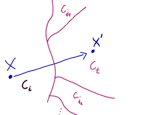
The attacks in this notebook constrain the perturbation by a pixel-space $L_\infty$ budget:
$$ \|x' - x\|_\infty \leq \epsilon. $$
This means no pixel channel may move by more than $\epsilon$ after converting the normalized tensor back to the valid pixel interval $[0,1]$. The code performs updates in normalized tensor coordinates, so $\epsilon$ and step sizes are divided by the per-channel standard deviation before applying gradient steps. After each projected update, the adversarial image is clipped back to the valid normalized image range.
This is why the perturbations can be visually small while still having a large effect. In high-dimensional image spaces, many tiny coordinate-wise changes can align with a loss-increasing direction. This is the phenomenon emphasized by Goodfellow et al. [2] and discussed from a high-dimensional viewpoint by Dube [4].
The notebook demonstrates three untargeted attacks from the standard adversarial-example literature: FGSM [2], I-FGSM/BIM [3], and PGD [5]. Each attack increases the classification loss with respect to the true label.
FGSM maximizes a first-order approximation of the loss under an $L_\infty$ constraint:
$$ \max_{\|\delta\|_\infty \leq \epsilon} J(\theta, x+\delta, y) \approx J(\theta, x, y)+\nabla_x J(\theta,x,y)^T\delta. $$
The maximizer of the linearized problem is the signed gradient direction:
$$ x'=x+\epsilon\,\operatorname{sign}(\nabla_x J(\theta,x,y)). $$
This is why FGSM is a one-step $L_\infty$ attack. It is computationally cheap and theoretically clear, but it only follows the loss surface at the original point. An $L_2$ attack would use a different constraint and therefore a different update direction.
I-FGSM, also called the Basic Iterative Method, repeats smaller FGSM-style steps and projects the result back into the allowed $L_\infty$ ball after each step:
$$ x_0'=x, \qquad x_{k+1}'=\operatorname{Clip}_{x,\epsilon}\left(x_k' + \alpha\,\operatorname{sign}(\nabla_{x_k'}J(\theta,x_k',y))\right). $$
This re-computes the gradient at each perturbed point, so it is usually stronger than one-step FGSM for the same $\epsilon$ budget.
PGD adds random initialization inside the $L_\infty$ ball before the iterative updates:
$$ x_0'=x+U(-\epsilon,\epsilon), $$
then applies the same projected signed-gradient idea. Random starts make PGD a stronger evaluation because the attack is less dependent on a single starting point. In this notebook, PGD uses 40 iterations, step size $\alpha=\epsilon/10$, and 3 random restarts, keeping the restart with the largest final cross-entropy loss. This makes PGD the main robustness stress test in the notebook.
Implementation of FGSM, I-FGSM, and PGD
The attack functions are wrapped by a decorator that runs the attack for each selected $\epsilon$, records accuracy, stores example images, and optionally builds confusion matrices. The evaluated $\epsilon$ values are 0.0, 0.0025, 0.005, 0.0075, 0.01, 0.02, 0.03, and 0.04 in pixel-space units.
############################# PLOTTER of IMAGES ##################################################
classes = ('plane', 'car', 'bird', 'cat', 'deer', 'dog', 'frog', 'horse', 'ship', 'truck')
def cifar_norm_tensors(device):
mean = torch.tensor(ACTIVE_MEAN, device=device).view(1, 3, 1, 1)
std = torch.tensor(ACTIVE_STD, device=device).view(1, 3, 1, 1)
return mean, std
def clamp_cifar_normalized(tensor):
mean, std = cifar_norm_tensors(tensor.device)
lower = (0.0 - mean) / std
upper = (1.0 - mean) / std
return torch.max(torch.min(tensor, upper), lower)
def eps_cifar_normalized(eps, tensor):
_, std = cifar_norm_tensors(tensor.device)
return eps / std
def pixel_linf_delta_normalized(original, adversarial):
"""Return max pixel-space Linf change for normalized tensors."""
_, std = cifar_norm_tensors(original.device)
return ((adversarial - original) * std).abs().amax().item()
def im_convert_2(tensor):
"""Denormalisation"""
image = tensor.detach().cpu() if torch.is_tensor(tensor) else torch.as_tensor(tensor)
mean = torch.tensor(ACTIVE_MEAN).view(3, 1, 1)
std = torch.tensor(ACTIVE_STD).view(3, 1, 1)
image = image * std + mean
image = image.permute(1, 2, 0).numpy().clip(0, 1)
return image
def plotter(imgs, probas, classes, epsilons):
"""Plot adversarial samples with non-overlapping compact labels."""
if not imgs:
print("No attack images to plot.")
return
rows = len(imgs)
cols = max(1, max(len(row) for row in imgs))
fig_width = max(15.5, cols * 2.75)
fig_height = max(6.0, rows * 2.25)
fig, axes = plt.subplots(
rows,
cols,
figsize=(fig_width, fig_height),
squeeze=False,
constrained_layout=True,
)
fig.set_constrained_layout_pads(w_pad=0.08, h_pad=0.06, wspace=0.08, hspace=0.10)
for ax in axes.ravel():
ax.set_axis_off()
for i, row in enumerate(imgs):
eps_label = epsilons[i] if i < len(epsilons) else i
for j, item in enumerate(row):
ax = axes[i, j]
ax.set_axis_on()
ax.set_xticks([])
ax.set_yticks([])
if j == 0:
ax.set_ylabel(f"Eps: {eps_label}", fontsize=16, rotation=90, labelpad=8)
if len(item) == 4:
true_label, clean_pred, adv_pred, ex = item
title_top = f"{classes[adv_pred]} ({classes[true_label]})"
title_bottom = f"{classes[clean_pred]} | {probas[i][j]:.1f}%"
is_correct = adv_pred == true_label
else:
true_label, adv_pred, ex = item
title_top = f"{classes[adv_pred]} ({classes[true_label]})"
title_bottom = f"{probas[i][j]:.1f}%"
is_correct = adv_pred == true_label
ax.set_title(
f"{title_top}\\n{title_bottom}",
color=("dodgerblue" if is_correct else "deeppink"),
fontsize=18.0,
pad=4,
loc="center",
)
ax.imshow(im_convert_2(ex))
for spine in ax.spines.values():
spine.set_linewidth(0.6)
spine.set_color("#999999")
plt.show()
#################################### ATTACK DECORATOR ####################################################
def main_attack(
model,
device,
test_loader,
epsilons,
matrix=False,
inference_model=None,
cpu_workers=None,
row_block_size=None,
):
def decorator(func):
def wrapper(*args, **kwargs):
"""Run an untargeted attack and aggregate metrics with process-based row blocks."""
if "assemble_confusion_matrix_row_blocks" not in globals():
raise RuntimeError("Run the confusion-matrix helper cell before adversarial attacks.")
if "make_sequential_loader_like" not in globals():
raise RuntimeError("Run the single-process DataLoader helper cell before adversarial attacks.")
# `model` must remain the differentiable PyTorch model used for gradients.
# `eval_model` may be PyTorch or TensorRT and is used only for scoring.
eval_model = inference_model if inference_model is not None else model
workers = ATTACK_CPU_WORKERS if cpu_workers is None else int(cpu_workers)
row_size = ATTACK_ROW_BLOCK_SIZE if row_block_size is None else row_block_size
eval_loader = make_sequential_loader_like(test_loader, batch_size=getattr(test_loader, "batch_size", None) or 32)
model.to(device)
model.eval()
if hasattr(eval_model, "to"):
eval_model.to(device)
if hasattr(eval_model, "eval"):
eval_model.eval()
accuracies = []
examples = []
probs = []
for eps in epsilons:
label_blocks = []
pred_blocks = []
adv_examples = []
x_probs = []
max_linf_delta = 0.0
loader_iter = tqdm(eval_loader, desc=f"eps={eps}", leave=False, dynamic_ncols=True) if tqdm is not None else eval_loader
for img, target in loader_iter:
img = img.clone().detach().to(device, non_blocking=True)
target = target.clone().detach().to(device, non_blocking=True)
with torch.no_grad(), torch.autocast(device_type=device.type, dtype=torch.float16, enabled=(device.type == "cuda")):
output = eval_model(img)
init_pred = output.argmax(1)
if eps == 0.0:
perturbed_img = img.detach()
else:
perturbed_img = func(model, img, target, eps, *args, **kwargs)
if perturbed_img.shape != img.shape:
raise RuntimeError(f"Attack returned shape {tuple(perturbed_img.shape)}, expected {tuple(img.shape)}")
perturbed_img = clamp_cifar_normalized(perturbed_img).detach()
batch_linf_delta = pixel_linf_delta_normalized(img, perturbed_img)
max_linf_delta = max(max_linf_delta, batch_linf_delta)
if batch_linf_delta > float(eps) + 2e-5:
raise RuntimeError(
f"{func.__name__} exceeded the pixel-space Linf budget: "
f"got {batch_linf_delta:.6f}, eps={float(eps):.6f}"
)
with torch.no_grad(), torch.autocast(device_type=device.type, dtype=torch.float16, enabled=(device.type == "cuda")):
output = eval_model(perturbed_img)
output_probs = F.softmax(output.float(), dim=1)
x_pred_prob = np.round(output_probs.max(dim=1).values.detach().cpu().numpy() * 100, 4)
final_pred = output.argmax(1)
label_blocks.append(target.detach().cpu().numpy().astype(np.int64, copy=False))
pred_blocks.append(final_pred.detach().cpu().numpy().astype(np.int64, copy=False))
remaining_examples = 7 - len(adv_examples)
if remaining_examples > 0:
success_idx = ((init_pred == target) & (final_pred != target)).nonzero(as_tuple=False).flatten().tolist()
fallback_idx = list(range(target.size(0)))
chosen = []
for idx in success_idx + fallback_idx:
if idx not in chosen:
chosen.append(idx)
if len(chosen) >= remaining_examples:
break
target_cpu = target.detach().cpu().numpy()
init_cpu = init_pred.detach().cpu().numpy()
final_cpu = final_pred.detach().cpu().numpy()
adv_cpu = perturbed_img.detach().cpu()
for idx in chosen:
adv_examples.append((int(target_cpu[idx]), int(init_cpu[idx]), int(final_cpu[idx]), adv_cpu[idx]))
x_probs.append(float(x_pred_prob[idx]))
labels_all = np.concatenate(label_blocks) if label_blocks else np.array([], dtype=np.int64)
preds_all = np.concatenate(pred_blocks) if pred_blocks else np.array([], dtype=np.int64)
conf_mat = assemble_confusion_matrix_row_blocks(
labels_all,
preds_all,
num_classes=len(classes),
workers=workers,
row_block_size=row_size,
)
correct = int(np.trace(conf_mat))
total_images = int(labels_all.size)
acc = correct / float(max(total_images, 1))
print("Epsilon: {} Test Accuracy = {} / {} = {:.4f}".format(eps, correct, total_images, acc))
print(f"Attack metric assembly: {total_images} rows, {min(workers, max(total_images, 1))} CPU workers; DataLoader workers=0")
if eps != 0.0:
print(f"Max pixel-space Linf delta observed: {max_linf_delta:.6f} <= eps {float(eps):.6f}")
accuracies.append(acc)
examples.append(adv_examples)
probs.append(x_probs)
print(' ')
if matrix:
plot_confusion_matrix(conf_mat, figsize=(8, 6), label_fontsize=13, axis_fontsize=12)
return accuracies, examples, probs
return wrapper
return decorator
Load Test Images for Attacks
The attack loader uses deterministic test images with batch size 8. This small batch size is a memory choice: ConvNeXt-Small at 224x224 requires gradients with respect to the input image, so attack evaluation is heavier than ordinary inference.
ATTACK_BATCH_SIZE = 8 # ConvNeXt-Small 224x224 attacks need gradient memory; use 4 if CUDA OOM persists.
ATTACK_EPSILONS = [0.0, 0.0025, 0.005, 0.0075, 0.01, 0.02, 0.03, 0.04]
ATTACK_SHOW_MATRICES = True
ATTACK_PGD_ITERS = 40
ATTACK_PGD_ALPHA_DIVISOR = 10
ATTACK_PGD_RESTARTS = 3
if device.type == "cuda":
torch.cuda.empty_cache()
_attack_loader_workers = 0
test2_loader = torch.utils.data.DataLoader(
test_dataset,
batch_size=ATTACK_BATCH_SIZE,
shuffle=False,
num_workers=_attack_loader_workers,
pin_memory=pin_memory,
persistent_workers=_attack_loader_workers > 0,
)
print(f"Attack batch size: {ATTACK_BATCH_SIZE}")
print(f"Attack epsilons: {ATTACK_EPSILONS}")
print(f"Attack DataLoader workers: {_attack_loader_workers}; CPU row-block workers: {globals().get('ATTACK_CPU_WORKERS', 1)}")
print(f"PGD: steps={ATTACK_PGD_ITERS}, alpha=eps/{ATTACK_PGD_ALPHA_DIVISOR}, restarts={ATTACK_PGD_RESTARTS}")
FGSM
FGSM uses one signed-gradient step:
$$ x'=x+\epsilon\,\operatorname{sign}(\nabla_x J(x, y_{true})). $$
torch.autograd.grad computes the derivative of the loss with respect to the input image. The saved source run starts from clean accuracy 0.9879. Under FGSM, accuracy declines gradually: 0.7770 at $\epsilon=0.0025$, 0.6963 at $\epsilon=0.005$, 0.6236 at $\epsilon=0.01$, and 0.5020 at $\epsilon=0.04$.
This curve is a useful baseline. FGSM exposes vulnerability, but because it is a single linearized step, it does not fully exploit the local loss landscape.
epsilons = ATTACK_EPSILONS
@main_attack(attack_model, device, test2_loader, epsilons, matrix=ATTACK_SHOW_MATRICES, inference_model=inference_model)
def fgsm(model, img, target, eps):
'''FGSM algorithm'''
img_adv = img.clone().detach().to(device)
img_adv.requires_grad = True
output = model(img_adv)
loss = F.cross_entropy(output, target)
grad = torch.autograd.grad(loss, img_adv, retain_graph=False, create_graph=False)[0]
eps_norm = eps_cifar_normalized(eps, img_adv)
perturb = img_adv + eps_norm * grad.sign()
perturbed_img = clamp_cifar_normalized(perturb).detach()
return perturbed_img
accuracies_fgsm, imgs_fgsm, probas_fgsm = fgsm()


Iterative FGSM
I-FGSM repeats projected signed-gradient steps:
$$ x_{k+1}'=\operatorname{Clip}_{x,\epsilon}\left(x_k' + \alpha\,\operatorname{sign}(\nabla_{x_k'}J(x_k', y_{true}))\right), $$
where $\operatorname{Clip}_{x,\epsilon}$ keeps the perturbation inside the $L_\infty$ ball around the original image. In the current implementation, the attack uses iters = 5, so the step size is $\alpha=\epsilon/5$.
Compared with FGSM, I-FGSM is much stronger because the model is relinearized after each small step. In the saved run, accuracy falls to 0.4476 at $\epsilon=0.0025$, 0.1282 at $\epsilon=0.005$, 0.0078 at $\epsilon=0.01$, and is effectively zero at larger budgets.
epsilons = ATTACK_EPSILONS
@main_attack(attack_model, device, test2_loader, epsilons, matrix=ATTACK_SHOW_MATRICES, inference_model=inference_model)
def I_fgsm(model, img, target, eps, iters):
'''I-FGSM algorithm'''
img_adv = img.clone().detach().to(device)
eps_norm = eps_cifar_normalized(eps, img_adv)
alpha = eps_norm / max(iters, 1)
perturbed_img = img_adv.detach()
for _ in range(iters):
img_adv = img_adv.detach().requires_grad_(True)
output = model(img_adv)
loss = F.cross_entropy(output, target)
grad = torch.autograd.grad(loss, img_adv, retain_graph=False, create_graph=False)[0]
perturbed = img_adv + alpha * grad.sign()
x_adv = torch.min(torch.max(perturbed, img - eps_norm), img + eps_norm)
img_adv = clamp_cifar_normalized(x_adv).detach()
perturbed_img = img_adv
return perturbed_img
iters = 5
accuracies_I5_fgsm, imgs_I5_fgsm, probas_I5_fgsm = I_fgsm(iters)


The I-FGSM results show that high clean accuracy does not imply adversarial robustness. The attack does not need to make images visually unrecognizable; it only needs to move them across the model's learned decision boundary. As $\epsilon$ grows, true positives are progressively replaced by false negatives and cross-class confusions.
This is the point where the notebook changes from classification performance to robustness analysis. The model is still the same trained ConvNeXt99 checkpoint; only the input construction has changed.
PGD
PGD repeats the signed-gradient step and projects the result back into the intersection of the allowed perturbation ball and valid image range:
$$ x_{k+1}'=\Pi_{B_\epsilon(x)\cap[0,1]^d}\left(x_k' + \alpha\,\operatorname{sign}(\nabla_{x_k'}J(\theta,x_k',y))\right). $$
With random initialization,
$$ x_0'=x+U(-\epsilon,\epsilon). $$
Here $B_\epsilon(x)$ is the pixel-space $L_\infty$ ball around the original image. The code carries out the update in normalized tensor coordinates and clips back to the valid normalized pixel bounds. The saved evaluation uses 40 PGD steps, $\alpha=\epsilon/10$, and 3 random restarts. This is the strongest attack tested in the notebook and the best indicator here of non-robustness under white-box evaluation.
epsilons = ATTACK_EPSILONS
@main_attack(attack_model, device, test2_loader, epsilons, matrix=ATTACK_SHOW_MATRICES, inference_model=inference_model)
def PGD(model, img, target, eps, iters=40, alpha_divisor=10, restarts=3, random_init=True):
"""Untargeted multi-restart Linf PGD.
Epsilon and alpha are specified in pixel-space units. The attack is carried
out in normalized tensor space, then projected back to the pixel-space Linf
ball around the original image after every step.
"""
img = img.clone().detach().to(device)
eps_norm = eps_cifar_normalized(eps, img)
alpha_norm = eps_cifar_normalized(eps / max(alpha_divisor, 1), img)
restarts = max(int(restarts), 1)
iters = max(int(iters), 1)
best_adv = img.detach().clone()
best_loss = torch.full((img.size(0),), -float("inf"), device=device)
for _ in range(restarts):
if random_init:
img_adv = img + torch.empty_like(img).uniform_(-1, 1) * eps_norm
img_adv = clamp_cifar_normalized(img_adv).detach()
else:
img_adv = img.detach().clone()
for _ in range(iters):
img_adv = img_adv.detach().requires_grad_(True)
output = model(img_adv)
losses = F.cross_entropy(output, target, reduction="none")
grad = torch.autograd.grad(losses.sum(), img_adv, retain_graph=False, create_graph=False)[0]
stepped = img_adv.detach() + alpha_norm * grad.sign()
delta = torch.max(torch.min(stepped - img, eps_norm), -eps_norm)
img_adv = clamp_cifar_normalized(img + delta).detach()
with torch.no_grad():
final_losses = F.cross_entropy(model(img_adv), target, reduction="none")
improve = final_losses > best_loss
best_loss = torch.where(improve, final_losses, best_loss)
best_adv = torch.where(improve.view(-1, 1, 1, 1), img_adv, best_adv)
return best_adv.detach()
pgd_iters = ATTACK_PGD_ITERS
pgd_alpha_divisor = ATTACK_PGD_ALPHA_DIVISOR
pgd_restarts = ATTACK_PGD_RESTARTS
accuracies_I40_proj, imgs_I40_proj, probas_I40_proj = PGD(
iters=pgd_iters,
alpha_divisor=pgd_alpha_divisor,
restarts=pgd_restarts,
random_init=True,
)


PGD is stronger than I-FGSM here because it uses more iterations, random starts, and keeps the adversarial example that maximizes the final loss. In the saved source outputs, PGD reduces accuracy from the clean 0.9879 to 0.0582 already at $\epsilon=0.0025$ and to 0.0000 from $\epsilon=0.005$ onward.
This result is consistent with the broader adversarial-robustness literature: standard high-accuracy training, even with strong data augmentation and distillation, does not by itself produce robustness against optimized white-box attacks. Robustness usually requires adversarial training or related robust optimization methods, and it can trade off with standard accuracy [5,6].
Accuracy as a Function of $\epsilon$
The next plot collects the completed attack curves. It should be read as a robustness curve: the faster a line falls, the less stable the classifier is under that attack family.
fig, ax = plt.subplots(figsize=(10, 8))
x_values = globals().get("epsilons", globals().get("ATTACK_EPSILONS", []))
curves = [
("accuracies_fgsm", "FGSM", "blueviolet"),
("accuracies_I5_fgsm", "Iterative_5-FGSM", "deeppink"),
("accuracies_I40_proj", "PGD-40, alpha=eps/10, 3 restarts", "dodgerblue"),
]
plotted = 0
missing = []
for var_name, label, color in curves:
values = globals().get(var_name)
if values is None:
missing.append(var_name)
continue
ax.plot(x_values[:len(values)], values, c=color, marker='o', label=label, linewidth=2.0)
plotted += 1
ax.set(xlabel=r"$\epsilon$", ylabel="Accuracy")
if plotted:
ax.legend()
plt.show()
else:
plt.close(fig)
print("No completed attack curves to plot yet.")
if missing:
print("Missing attack results:", ", ".join(missing))
print("Run the corresponding attack cells before plotting them.")

The accuracy curves compare the attacks over the same $\epsilon$ values. FGSM is the weakest because it uses a single linearized step. I-FGSM is stronger because it repeatedly updates and projects. PGD is strongest in this notebook because it combines iterative projection with random restarts.
The image grids below show examples at increasing $\epsilon$. The labels above each image report the adversarial prediction and confidence. These examples are not meant to replace the full test-set curves; they are qualitative illustrations of how small perturbation budgets can produce confident wrong predictions.
FGSM
def plotter_no_clean(imgs, probas, classes, epsilons):
"""Plot adversarial samples with compact labels."""
if not imgs:
print("No attack images to plot.")
return
rows = len(imgs)
cols = max(1, max(len(row) for row in imgs))
fig, axes = plt.subplots(
rows,
cols,
figsize=(max(16.5, cols * 2.95), max(6.0, rows * 2.30)),
squeeze=False,
constrained_layout=True,
)
fig.set_constrained_layout_pads(w_pad=0.10, h_pad=0.07, wspace=0.10, hspace=0.12)
for ax in axes.ravel():
ax.set_axis_off()
for i, row in enumerate(imgs):
eps_label = epsilons[i] if i < len(epsilons) else i
for j, item in enumerate(row):
ax = axes[i, j]
ax.set_axis_on()
ax.set_xticks([])
ax.set_yticks([])
if j == 0:
ax.set_ylabel(f"Eps: {eps_label}", fontsize=16, rotation=90, labelpad=8)
if len(item) == 4:
true_label, base_pred, adv_pred, ex = item
title = f"{classes[adv_pred]} ({classes[true_label]})\n{classes[base_pred]} | {probas[i][j]:.1f}%"
is_correct = adv_pred == true_label
else:
true_label, adv_pred, ex = item
title = f"{classes[adv_pred]} ({classes[true_label]})\n{probas[i][j]:.1f}%"
is_correct = adv_pred == true_label
ax.set_title(
title,
color=("dodgerblue" if is_correct else "deeppink"),
fontsize=18.0,
pad=4,
)
ax.imshow(im_convert_2(ex))
for spine in ax.spines.values():
spine.set_linewidth(0.6)
spine.set_color("#999999")
plt.show()
if "imgs_fgsm" in globals() and "probas_fgsm" in globals():
plotter_no_clean(imgs_fgsm, probas_fgsm, classes, epsilons)
else:
print("FGSM examples are not available yet. Run the FGSM attack cell first.")

I-FGSM
The I-FGSM image grid should be compared with the FGSM grid at the same $\epsilon$ values. The visual changes can still be small, but the predictions change much more aggressively because each step follows a newly computed gradient.
def plotter_no_clean(imgs, probas, classes, epsilons):
"""Plot adversarial samples with compact labels."""
if not imgs:
print("No attack images to plot.")
return
rows = len(imgs)
cols = max(1, max(len(row) for row in imgs))
fig, axes = plt.subplots(
rows,
cols,
figsize=(max(16.5, cols * 2.95), max(6.0, rows * 2.30)),
squeeze=False,
constrained_layout=True,
)
fig.set_constrained_layout_pads(w_pad=0.10, h_pad=0.07, wspace=0.10, hspace=0.12)
for ax in axes.ravel():
ax.set_axis_off()
for i, row in enumerate(imgs):
eps_label = epsilons[i] if i < len(epsilons) else i
for j, item in enumerate(row):
ax = axes[i, j]
ax.set_axis_on()
ax.set_xticks([])
ax.set_yticks([])
if j == 0:
ax.set_ylabel(f"Eps: {eps_label}", fontsize=16, rotation=90, labelpad=8)
if len(item) == 4:
true_label, base_pred, adv_pred, ex = item
title = f"{classes[adv_pred]} ({classes[true_label]})\n{classes[base_pred]} | {probas[i][j]:.1f}%"
is_correct = adv_pred == true_label
else:
true_label, adv_pred, ex = item
title = f"{classes[adv_pred]} ({classes[true_label]})\n{probas[i][j]:.1f}%"
is_correct = adv_pred == true_label
ax.set_title(
title,
color=("dodgerblue" if is_correct else "deeppink"),
fontsize=18.0,
pad=4,
)
ax.imshow(im_convert_2(ex))
for spine in ax.spines.values():
spine.set_linewidth(0.6)
spine.set_color("#999999")
plt.show()
if "imgs_I5_fgsm" in globals() and "probas_I5_fgsm" in globals():
plotter_no_clean(imgs_I5_fgsm, probas_I5_fgsm, classes, epsilons)
else:
print("I-FGSM examples are not available yet. Run the I-FGSM attack cell first.")

PGD Attack
The PGD image grid shows the strongest attack setting used here: 40 steps, $\alpha=\epsilon/10$, and 3 random restarts. Because the attack keeps the highest-loss restart, these examples represent a harder white-box robustness test than the single-start iterative attack.
def plotter_no_clean(imgs, probas, classes, epsilons):
"""Plot adversarial samples with compact labels."""
if not imgs:
print("No attack images to plot.")
return
rows = len(imgs)
cols = max(1, max(len(row) for row in imgs))
fig, axes = plt.subplots(
rows,
cols,
figsize=(max(16.5, cols * 2.95), max(6.0, rows * 2.30)),
squeeze=False,
constrained_layout=True,
)
fig.set_constrained_layout_pads(w_pad=0.10, h_pad=0.07, wspace=0.10, hspace=0.12)
for ax in axes.ravel():
ax.set_axis_off()
for i, row in enumerate(imgs):
eps_label = epsilons[i] if i < len(epsilons) else i
for j, item in enumerate(row):
ax = axes[i, j]
ax.set_axis_on()
ax.set_xticks([])
ax.set_yticks([])
if j == 0:
ax.set_ylabel(f"Eps: {eps_label}", fontsize=16, rotation=90, labelpad=8)
if len(item) == 4:
true_label, base_pred, adv_pred, ex = item
title = f"{classes[adv_pred]} ({classes[true_label]})\n{classes[base_pred]} | {probas[i][j]:.1f}%"
is_correct = adv_pred == true_label
else:
true_label, adv_pred, ex = item
title = f"{classes[adv_pred]} ({classes[true_label]})\n{probas[i][j]:.1f}%"
is_correct = adv_pred == true_label
ax.set_title(
title,
color=("dodgerblue" if is_correct else "deeppink"),
fontsize=18.0,
pad=4,
)
ax.imshow(im_convert_2(ex))
for spine in ax.spines.values():
spine.set_linewidth(0.6)
spine.set_color("#999999")
plt.show()
if "imgs_I40_proj" in globals() and "probas_I40_proj" in globals():
plotter_no_clean(imgs_I40_proj, probas_I40_proj, classes, epsilons)
else:
print("PGD examples are not available yet. Run the PGD attack cell first.")

Results and Interpretation
The final clean classifier is strong: the saved ConvNeXt99 checkpoint reaches 98.79% clean test accuracy, with best TTA/basic test accuracy 0.9879. The two-step training path is effective for standard CIFAR-10 classification. AirBench96 gives a fast 0.9615 TTA teacher/baseline, and ImageNet-pretrained ConvNeXt-Small with light distillation raises performance close to the 0.99 target.
The training analysis is important for interpreting this result. The pretrained ConvNeXt backbone supplies most of the representation power immediately, as shown by 0.9752 TTA after one epoch. The later epochs improve more slowly, with the best value arriving around epoch 27. The final epoch is not the best epoch, so checkpointing by TTA test accuracy is necessary. The model eventually fits the clean training set exactly, but the test curve still improves slightly under the low learning-rate cosine schedule and regularized fine-tuning.
The class-wise results are also informative. Frog, deer, ship, horse, and car are above 99%; cat and dog are lower. This suggests the remaining clean errors are concentrated in visually similar or ambiguous CIFAR-10 categories rather than spread uniformly across the dataset.
The adversarial results tell a different story. FGSM reduces accuracy but leaves about half the test set correctly classified at $\epsilon=0.04$. I-FGSM is much stronger and nearly eliminates accuracy at larger budgets. PGD-40 with $\alpha=\epsilon/10$ and 3 random restarts is strongest, reaching zero accuracy from $\epsilon=0.005$ in the saved run. This gap between clean accuracy and adversarial robustness is the central methodological lesson of the notebook: a model can generalize very well on the natural test distribution while remaining brittle under small, optimized perturbations.
The interpretation follows the literature already cited in the notebook. ConvNeXt [1] explains the clean-accuracy architecture choice. Goodfellow et al. [2] motivate the signed-gradient view of adversarial examples. Kurakin et al. [3] motivate iterative attacks in image models. Dube [4] supports the high-dimensional interpretation of small coordinate-wise changes. Tsipras et al. [5] and Deniz et al. [6] frame the tension between standard accuracy, robustness, and training objectives. The notebook's empirical result fits that story: modern pretraining and distillation improve clean CIFAR-10 accuracy, but robust behavior requires explicit robust optimization rather than ordinary fine-tuning alone.
References
[1] Liu, Z. et al., 2022. A ConvNet for the 2020s. Proceedings of the IEEE/CVF Conference on Computer Vision and Pattern Recognition.
[2] Goodfellow, I.J., Shlens, J. and Szegedy, C., 2014. Explaining and harnessing adversarial examples. arXiv preprint arXiv:1412.6572.
[3] Kurakin, A., Goodfellow, I. and Bengio, S., 2016. Adversarial examples in the physical world. arXiv preprint arXiv:1607.02533.
[4] Dube, S., 2018. High dimensional spaces, deep learning and adversarial examples. arXiv preprint arXiv:1801.00634.
[5] Tsipras, D., Santurkar, S., Engstrom, L., Turner, A. and Madry, A., 2018. Robustness may be at odds with accuracy. arXiv preprint arXiv:1805.12152.
[6] Deniz, O., Pedraza, A., Vallez, N. et al. Robustness to adversarial examples can be improved with overfitting. Int. J. Mach. Learn. & Cyber. 11, 935-944 (2020).
