Method of Lines for Black-Scholes Implicit
IMPLICIT METHOD of LINES (MOL) for the BLACK-SCHOLES MODEL in PYTHON
There are various numerical schemes to solve PDEs. The finite difference and finite element or Galerkin methods are very popular. However, a semi-analytical approach called Method of Lines (MOL) allows for decent approximation accuracies. In this post, I show how to apply MOL to price European (EU) option based on the Black-Scholes model.
Let's consider the function $V=V(t,x)$ and its derivative $\partial_{t} = L(V)$.
Method of Lines (MOL) amounts to the discretisation of PDE in space. Thus we set up a grid of points ${x_{i}}$. Then for each ${x_{i}}$, the individual ODE is solved along a time. Therefore the PDE is expressed in the form of one variable, $t$, instead of $x$ and $t$ as it is in case of finite difference or finite element methods. Namely, the system of ODEs is coupled by linear or non-linear operator $\mathbb{L}$ nad solved. In case of linear PDE, $\mathbb{L}$ is simply a matrix. For the non-linear, there is a matrix as well but depending itself on $V$ like in the Burger's eqn. Linearity has enormous advantages as far as the numerical approach is concerned.
Hence, we evaluate in terms of components of vector $\vec{v}$ which depends on time, $\overrightarrow{v}_{i}=\overrightarrow{v}(t,x_{i})$, with each component labeled by index $i$. So, in the general case, we can write $$\frac{d\overrightarrow{v}_{i}}{dt}=\mathbb{L}(\overrightarrow{v})$$ For the linear case we re-write our eqn as dot product of matrix $\mathbb{L}$ onto vector $\overrightarrow{v}$ $$\frac{d\overrightarrow{v}_{i}}{dt}=\sum_{j} L_{ji} \overrightarrow{v}_{j}=\mathbb{L}(\overrightarrow{v})$$
For a better illustration, for example, the simple advection eqn $\frac{\partial U}{\partial t}=c \frac{\partial U}{\partial x}$ for MOL purposes is written as $\frac{d\overrightarrow{u}}{\text{dt}}=\mathbb{L}\left(\overrightarrow{u}\right)=c\,\mathbb{D}\cdot\vec{u}$. Namely, there is an ODE for each component of $\vec{U}$, that is $u_{1}, u_{2},...,u_{m}$. Again for $Nx$ grid points we have $Nx$ ODEs coupled by linear or non-linear operator $\mathbb L$. The next step is to apply explicit or implicit methods such as Runge-Kutta or Trapezoidal, respectively.
In this notebook I will demonstrate how to solve BS model using implicit Hermite scheme that has fourth order accuracy.
But what are the advantages of the implicit method in general?
Technically, Trapezoidal (2 order), Hermite (4 order) or Lotkin (6 order) are integrators on equidistant nodes constructed through interpolation of a polynomial using the method of undetermined coefficients. To set up Hermite or Lotkin, we derivatives as well. The Lotkin formula encompasses trapezoidal, Hermite and Lotkin terms consecutively $$\int_a^b f x \, dx\simeq \frac{1}{2} h (f(a)+f(b))+\frac{1}{10} h^2 \left(f'(a)- f'(b)\right)+\frac{1}{120} h^3 \left(f''(a)+f''(b)\right)$$
The crux is that if we change $\int_a^b f x \, dx\longrightarrow \int_b^a f x \, dx$, the formula stays the same. That is why when you consider dynamical systems, the symmetry is kept and, in turn, energy is conserved (for linear systems, the symplectic structure as well). In consequence, the system is unconditionally stable and exhibits higher accuracy than explicit counterparts.
Now, as we know why implicit schemes are superior, we can come back to PDE.
Following our simple advection equation $\frac{\partial U}{\partial t}=c \frac{\partial U}{\partial x}$, by Fundamental Theorem of Calculus we integrate it forward in time (remember that $U$ is vectorised) $$\overrightarrow{U}(t_{j+1})-\overrightarrow{U}(t_{j}) = \int_{j}^{j+1} \mathbb{L} (\overrightarrow{U}_{t}) \, dt$$ and approximate the integrand by Hermite integrator
$$\int _j^{(j+1)}\overrightarrow{U}tdt\simeq \text{$\Delta $t}\frac{\overrightarrow{U}^{(j)}+\overrightarrow{U}^{(j+1)}}{2}+\text{$\Delta $t}^2\frac{\overrightarrow{\dot{U}}^{(j)}+\overrightarrow{\dot{U}}^{(j+1)}}{12}$$
Since $\overset{\overrightarrow\cdot}{U}=\frac{d\overrightarrow{u}}{\text{dt}}=\mathbb{L}\cdot \overrightarrow{u}$, then we can write
$$\overrightarrow{U}^{(j+1)}=\overrightarrow{U}^{(j)}+\frac{1}{2}\text{$\Delta $t}\cdot\mathbb{L}\left(\overrightarrow{U}^{(j)}+\overrightarrow{U}^{(j+1)}\right)+\frac{1}{12}\text{$\Delta $t}\cdot\mathbb{L}\left(\overrightarrow{\dot{U}}^{(j+1)}+\overrightarrow{\dot{U}}^{(j+1)}\right) $$
Since we deal with the linear eqution we have an easy job (our machines too) $$\overrightarrow{U}^{(j+1)}=\overrightarrow{U}^{(j)}+\frac{1}{2}\text{$\Delta $t}\cdot\mathbb{L}\left(\overrightarrow{U}^{(j)}+\overrightarrow{U}^{(j+1)}\right)+\frac{1}{12}\text{$\Delta $t}\,\cdot\mathbb{L}\left(\mathbb{L}\,\overrightarrow{U}^{(j+1)}+\mathbb{L}\,\overrightarrow{U}^{(j+1)}\right) $$
$$\overrightarrow{U}^{(j+1)}=\overrightarrow{U}^{(j)}+\frac{1}{2}\text{$\Delta $t}\cdot\mathbb{L}\left(\overrightarrow{U}^{(j)}+\overrightarrow{U}^{(j+1)}\right)+\frac{1}{12}\text{$\Delta $t}\,\cdot\mathbb{L}^2\left(\overrightarrow{U}^{(j+1)}+\overrightarrow{U}^{(j+1)}\right) $$
Let's deploy time terms on the opposite sides of the equation (***) $$\left(\mathbb{I}+\frac{\text{$\Delta $t}^2 \mathbb{L}^2}{10}-\frac{\text{$\Delta $t} \mathbb{L}}{2}\right)\cdot\overrightarrow{U}^{(j+1)}=\left(\mathbb{I}+\frac{\text{$\Delta $t}^2 \mathbb{L}^2}{10}+\frac{\text{$\Delta $t} \mathbb{L}}{2}\right)\cdot\overrightarrow{U}^{(j+1)}$$
In general, we use Thomas algorithm to invert the above matrix or solve the system during each iteration $$\overrightarrow{U}^{(j+1)}=\left(\mathbb{I}+\frac{\text{$\Delta $t}^2 \mathbb{L}^2}{10}-\frac{\text{$\Delta $t} \mathbb{L}}{2}\right)^{-1}\cdot\left(\mathbb{I}+\frac{\text{$\Delta $t}^2 \mathbb{L}^2}{10}+\frac{\text{$\Delta $t} \mathbb{L}}{2}\right)\cdot\overrightarrow{U}^{(j)}$$ Luckily, we deal with the Black-Scholes equation that is linear. So, we can invert the LHS matrix beforehand, store it and as such use it in each iteration $$M= \left(\mathbb{I}+\frac{\text{$\Delta $t}^2 \mathbb{L}^2}{10}-\frac{\text{$\Delta $t} \mathbb{L}}{2}\right)^{-1}\cdot\left(\mathbb{I}+\frac{\text{$\Delta $t}^2 \mathbb{L}^2}{10}+\frac{\text{$\Delta $t} \mathbb{L}}{2}\right)$$ and within the loop $$\overrightarrow{U}^{(j+1)}=M\cdot\overrightarrow{U}^{(j)}$$
Black-Scholes (BS) equation
The Black-Scholes eqn is first order in time and second ordered in space parabolic linear equation, where $s$ is the price of the underlying asset and $K$ is a strike price, $\sigma$ represents volatility and $r$ the intrest rate. The value of option at time, $t$, before expiration, $T$, is from $$\frac{\partial V(t,s)}{\partial s}+\frac{1}{2} s^2 \sigma ^2 \frac{\partial ^2V(t,s)}{\partial s^2}+\frac{\partial V(t,s)}{\partial t}-\text{rV}(t,s)=0$$ with the following closed-form solution $$V(t,s)=\frac{1}{2} e^{-r T} \left(\frac{s e^{r T} \left(\text{erfc} \left(2 K \log +\left(2 r+\sigma ^2\right) (t-T)-2 (s \log )\right)\right)}{2 \sqrt{2} \sigma \sqrt{T-t}}-\frac{K e^{r t} \left(\text{erfc} \left(2 K \log +\left(2 r-\sigma ^2\right) (t-T)-2 (s \log )\right)\right)}{2 \sqrt{2} \sigma \sqrt{T-t}}\right)$$ Input data are the price of the underlying asset $s$, strike price $K$, time to maturity T, interest rate r, and volatility $\sigma$. The price of the call option is $V(t,s)$.
The BS equation is parabolic, and its variables depend upon the time and price of underplaying asset. This model assumes that the option pricing is a continuous function of time, and the underlying asset price follows the geometric Brownian motion described by SDE
$$\frac{dS_t}{S_t} = \mu dt + \sigma dW_t$$
That is why the BS equation can be derived from the Brownian process. As there is a deep connection between the Brownian process and the heat equation (Einstein relation), the original BS eqn can be easy transformed into the diffusion equation whose heat kernel evolves according to the normal distribution.
The BS eqn satisfies the terminal condition for the final pay-off $V(S_{t},T)=max(S_{t}-K,0)$. The Dirichlet boundary conditions (BCs) at $S_{t}=0$ is $V(0,t)=0$ and since $S_{t}\longrightarrow +\infty$ then the boundary at $S_{t, max}$ is $V(S_{t,max},t)=S_{t}-KE^{-r(T-t)}$.
MOL for the Black-Scholes equation
For $j = 0,1, ... Nt$, define the discrete time step $ \Delta t = \frac{T - t_0}{Nt} $ such that $t_j = t_0 + j \Delta t$. For $i = 0,1, ... Ns$, define the discrete space step $ \Delta x = \frac{x_2 - x_1}{Ns} $ such that $x_i = x_1 + i \Delta x$. The grid points have the form of $(t_0 + n \Delta t, x_1 + i \Delta x)$. At this point, we concern ourselves only with the values of $V(t,x)$ on the grid nodes. Therefore if $j's$ are for rows and $i's$ are for columns, we have the grid
$$ V(t_0 + j \Delta t, x_1 + i \Delta x) = V_{j,i} $$
We are interested in the value of an option, V, at $t_{0}$, which means that BS eqn is a backward in time. We know the values $V(T, S_{t})$ corresponding to the terminal conditions. The algorithm finds the values $V_{j}$ given the knowledge of the values $V_{j+1}$. For convenience, we can invert BS eqn by introducing a new variable $\tau = -t$ and change the variables in the PDE $$\frac{\partial V}{\partial t}=\frac{\partial V}{\partial \tau}\frac{\partial \tau}{\partial t}=\frac{\partial V}{\partial \tau}\frac{\partial}{\partial t}(T-t)=-\frac{\partial V}{\partial \tau}$$ Given that the terminal conditions become initial conditions, and the eqn becomes a forward problem $$\frac{\partial V(\tau,s)}{\partial \tau} =\frac{1}{2} s^2 \sigma ^2 \frac{\partial ^2V(\tau,s)}{\partial s^2}+\frac{\partial V(\tau,s)}{\partial s}-\text{rV}(\tau,s)=0$$
As one can observe, there two partial derivatives terms to discretise, first and second orders respectively, by means of central differences $$\frac{\partial V(\tau,s)}{\partial s} \approx \frac{V(\tau, s+\Delta s) - V(\tau, s-\Delta s)}{2\Delta s} + \frac{1}{6} V^{(3)} ds^2$$
However, the first and the last rows are populated by approximations of the form $$\frac{\partial^2 V(\tau,s)}{\partial s^2} \approx \frac{-3V(\tau,s) + 4V(\tau,s+\Delta s) - V(\tau,s+2\Delta s)}{ \Delta s^2} + \frac{1}{3} V^{(3)} ds^2$$
Analogically for the second derivative matrix
$$\frac{\partial^2 V(\tau,s)}{\partial s^2} \approx \frac{V(\tau,s+\Delta s) + V(\tau,s-\Delta s) - 2V(\tau,s)}{ \Delta s^2} + \frac{11}{12} V^{(4)} ds^2$$
$$\frac{\partial^2 V(\tau,s)}{\partial s^2} \approx \frac{2 V(\tau,s) -5 V(\tau,s+\Delta s) + 4V(\tau,s+2\Delta s) +3\Delta s}{ \Delta s^2} + \frac{11}{12} V^{(4)} ds^2$$ The last terms are the error terms.
Now we are able to set up the difference matrices in price, $S$ with shape $(Ns-2, Ns-2)$ because i=0 and i=Ns are accupied by lateral boundary conditions.
Note that I applied the second-order polynomials (uses three points) to obtain finite difference formulae. In addition, I put formulae from third-order polynomials in the first and last rows. This technique decreases the error of estimation considerably and accommodates boundary conditions in a pretty nice manner, which is not always apparent for approaches for BS aquation without log variable transformation.
As a result, the first and second derivative differentiation matrices have a form
$$\mathbb{D}^{(1)}=\frac{1}{2ds}\mathbb{L}^{(1)}=\frac{1}{2ds}\left(
\begin{array}{ccccc}
-3 & 2 & -1 & 0 & \cdots & 0 \\
-1 & 0 & 1 & 0 & 0 & 0 \\
0 & \ddots & \ddots & \ddots & \ddots & 0\\
\vdots & 0 & -1 & 0 & 1 & 0 \\
0 & 0 & 0 & -1 & 0 & 1 \\
0 & 0 & 0 & -1 & -2 & 3\\
\end{array}
\right)$$
and
$$\mathbb{D}^{(2)}=\frac{1}{2ds^2}\mathbb{L}^{(2)}=\frac{1}{2ds^2}\left(
\begin{array}{ccccc}
2 & -5 & 4 & -1 & \cdots & 0 \\
1 & -2 & 1 & 0 & 0 & 0 \\
0 & \ddots & \ddots & \ddots & \ddots & 0\\
\vdots & 0 & 1 & -2 & 1 & 0 \\
0 & 0 & 0 & 1 & -2 & 1 \\
0 & 0 & -1 & 4 & -5 & 2\\
\end{array}
\right)$$
, respectivelly.
Moreover
$$\mathbb{R} = r\left(
\begin{array}{ccccc}
1 & 0 & 0 & \cdots & 0 \\
0 & 1 & 0 & 0 & 0 \\
0 & 0 & 1 & 0 & 0 \\
0 & \ddots & \ddots & \ddots & 0 \\
\vdots & 0 & 0 & 1 & 0 \\
0 & 0 & 0 & 0 & 1 \\
\end{array}
\right)$$
Therefore we obtain a linear operator for Black-Scholes model as follows $$\mathbb{L}=\frac{1}{2}\sigma ^2S_i\mathbb{D}^{(2)}+\text{r} S_{i}\mathbb{D}^{(1)}-\mathbb{R}$$
We substitute this operator to (***) and populate matrix $V(\tau,s)$
Implementation
Following the above recipe we will compute the price of the EU option at $t_{0}$ for $K$=100, $S_{0}$=100, $T$=12/12, $r$=0.1, $\sigma$=0.2. Bear in mind that the matrix operator has dimensions $(Ns-1\, per\, Ns-1)$. The first and the last rows are for lateral boundaries.
import numpy as np
import matplotlib.pyplot as plt
from matplotlib import cm
%matplotlib inline
#!conda install -c conda-forge jupyterthemes
from jupyterthemes import jtplot
jtplot.style(theme="grade3", context="notebook", ticks=True, grid=True)
def mol_call_imp(S0, K, sig, r, Texpir, Ns, Nt, plotti=False):
"""Computes price of call be means of Method of Lines"""
#Set domain
S_max = 4*float(K)
S_min = float(K)/4
#Grids
S, ds = np.linspace(S_min,S_max, Ns, retstep=True)
T, dt = np.linspace(0, Texpir, Nt, retstep=True)
V = np.zeros((Ns,Nt))
Payoff = np.maximum(S-K,0)
B = np.zeros(Ns-2)
#Boundaries
V[:,0] = Payoff
upper = np.zeros_like(T)
lower = S_max - K * np.exp(-r* T[::-1])
#Matrix constructor
s = S[1:-1] #vector of stock values
s1= s[:, None] #add axis
ds2 = ds*ds
sig2 = sig*sig
D1 = np.zeros((Ns-2, Ns-2))
for i in range(0, Ns-3):
D1[i+1,i]=-1.
D1[i,i+1]=1.
D1[0,0]=-3.
D1[-1,-1]=3.
D1[0,2]=-1.
D1[0,1]=2.
D1[-1,-2]=-4
D1[-1,-3]=1.
#Firs derivative matrix
D1 = (r/(2*ds))*s1*D1
D2=np.zeros((Ns-2,Ns-2))
for i in range(0,Ns-2):
D2[i,i]=-2.
for i in range(0, Ns-3):
D2[i+1,i]=1.
D2[i,i+1]=1.
D2[0,1]=D2[-1,-2]=-2.
D2[0,1]=D2[-1,-2]=-5.
D2[0,2]=D2[-1,-3]=4.
D2[0,3]=D2[-1,-4]=-1.
D2[0,0]=D2[-1,-1]=2
#Second derivative matrix
D2 = (sig2/(2*(ds2)))*(s1**2)*D2
#Constant term matrix
D3 = -r*np.eye(Ns-2)
#Construction of operator
L = D2+D1+D3
II = np.eye(Ns-2)
#Hermite
M1 = II - (dt/2)*L + (dt**2/10)*(L@L)
M2 = II + (dt/2)*L + (dt**2/10)*(L@L)
M1inv = np.linalg.inv(M1)
M = M1inv@M2
#Solver of ODEs' system
for j in range(0, Nt-1):
V[1:-1,j+1] =np.dot(M,(V[1:-1,j]))
V[0,j+1] = upper[j]
V[-1,j+1] = lower[j]
oPrice = np.interp(S0, S, V[:,-1])
if plotti:
fig = plt.figure(figsize=(18,8))
ax1 = fig.add_subplot(121)
ax2 = fig.add_subplot(122, projection='3d')
ax1.plot(S, Payoff, color='deeppink',label="Payoff")
ax1.plot(S, V[:,-1], color='dodgerblue',label="BS curve")
ax1.set_xlim(50,150); ax1.set_ylim(0,40)
ax1.set_xlabel("S"); ax1.set_ylabel("price")
ax1.legend(loc='upper left'); ax1.set_title("BS price at t=0")
X, Y = np.meshgrid(T[::-1], S)
ax2.plot_surface(Y, X, V, cmap=cm.gist_ncar)
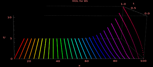
ax2.set_title("BS price surface")
ax2.set_xlabel("S"); ax2.set_ylabel("t"); ax2.set_zlabel("V")
ax2.view_init(30, -100)
plt.show()
#Remember to put analytic price of your option
print('The price of call option is: {} with error: {}'.format(oPrice, np.abs(oPrice - 13.269676584660893)))
Now we are ready to test our pricer and plot results
#Inputs
r = 0.1
sig = 0.2
S0 = 100.
K = 100.
Texpir = 1.
Ns = 300
Nt = 50

mol_call_imp(S0, K, sig, r, Texpir, Ns, Nt, plotti=True)

mol_call_imp(S0, K, sig, r, Texpir, 7000, 500, plotti=False)
What could be done more? Transformation of BS eqn to the heat equation would decrease the error since, in the heat equation, there is only one second derivative difference matrix, and it would be advisable to add the Lotkin term. Moreover, working on the log scale would improve the accommodation of boundary conditions. Another approach would be to build a MOL scheme backed by neural networks.
Thank you for reading, and you are welcome to visit other posts on my blog.
