DMD for El Nino
DMD for El Nino
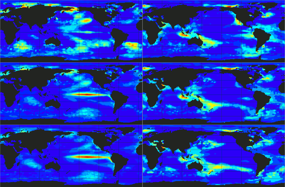
[If you want to omit theory and go directly to the code.]
Dynamic Mode Decomposition (DMD) is a data-driven method for fitting a low-dimensional linear evolution model to snapshot data from a dynamical system. If the columns of $X$ are measurements $x_0, x_1, \ldots, x_{m-2}$ and the columns of $X'$ are the shifted measurements $x_1, x_2, \ldots, x_{m-1}$, DMD looks for a linear operator $A$ such that
$$ x_{k+1} \approx A x_k. $$
The least-squares fit is
$$ A = \arg\min_A \|X' - AX\|_F = X'X^{\dagger}, $$
where $\|\cdot\|_F$ is the Frobenius norm and $X^{\dagger}$ is the Moore-Penrose pseudoinverse. In practice, $A$ is usually too large to form explicitly, so DMD computes its leading spectral information through a truncated SVD of $X$.
In this notebook, each state vector is a flattened sea-surface-temperature field. The code below follows the original exact-DMD workflow and uses the selected modes for reconstruction and visualization.
The connection with Koopman theory is useful but has to be stated carefully: DMD modes are not Koopman eigenfunctions. For direct measurements $g(x)=x$, DMD modes approximate Koopman modes for the chosen observable, while the DMD eigenvalues approximate Koopman eigenvalues under the sampling and observable assumptions described below.
Koopman viewpoint
Consider an autonomous continuous-time system
$$ \dot{x} = f(x), \qquad x \in X. $$
Let $F^t(x)$ denote its flow: the state reached after time $t$ when the initial condition is $x$. A scalar observable is a function $g:X\to\mathbb{C}$. The Koopman operator family acts on observables by composition with the flow,
$$ (\mathcal{K}^t g)(x) = g(F^t(x)). $$
For a discrete-time system
$$ x_{k+1}=F(x_k), $$
the one-step Koopman operator is
$$ (\mathcal{K}g)(x) = g(F(x)). $$
The operator is linear because, for observables $g_1,g_2$ and scalars $a,b$,
$$ \mathcal{K}(a g_1 + b g_2) = a\mathcal{K}g_1 + b\mathcal{K}g_2, $$
although the underlying dynamics $F$ may be nonlinear. The price is that $\mathcal{K}$ acts on a function space, usually infinite-dimensional.
A Koopman eigenfunction is a nonzero scalar observable $\varphi$ satisfying
$$ \mathcal{K}\varphi = \lambda \varphi $$
in discrete time, or
$$ \mathcal{K}^t\varphi = e^{\omega t}\varphi $$
in continuous time. The discrete eigenvalue is $\lambda$; the continuous-time eigenvalue is $\omega$. For uniformly sampled data with time step $\Delta t$, they are related by
$$ \omega = \frac{\log(\lambda)}{\Delta t}, $$
with the usual branch ambiguity of the complex logarithm.
For continuous-time systems, the infinitesimal generator $\mathcal{L}$ is distinct from the Koopman operator family. It satisfies
$$ (\mathcal{L}g)(x) = \nabla g(x)\cdot f(x). $$
If $\varphi$ is a generator eigenfunction, then
$$ \mathcal{L}\varphi = \nabla \varphi(x)\cdot f(x) = \omega\varphi(x). $$
This is the chain-rule equation often used to discuss Koopman eigenfunctions. It should not be confused with the discrete operator equation $\mathcal{K}\varphi=\lambda\varphi$.
Koopman modes, eigenfunctions, and DMD modes
For a vector-valued observable $g:X\to\mathbb{C}^p$, a Koopman mode expansion has the form
$$ g(x_k) = \mathcal{K}^k g(x_0) \approx \sum_{j=1}^{r} \lambda_j^k\,\varphi_j(x_0)\,v_j. $$
Here:
- $\varphi_j$ are Koopman eigenfunctions, which are scalar functions on state space.
- $\lambda_j$ are discrete-time Koopman eigenvalues.
- $v_j$ are Koopman modes, vectors in measurement space.
DMD estimates a finite-dimensional version of this expansion from data. With direct measurements $g(x)=x$, the DMD modes $\phi_j$ are approximations of Koopman modes $v_j$, not approximations of the scalar eigenfunctions $\varphi_j$. The DMD amplitudes $b_j$ play the role of the eigenfunctions evaluated at the initial condition, $\varphi_j(x_0)$, for the fitted data window.
This distinction matters when interpreting spatial plots. A plotted DMD mode is a spatial coefficient pattern. Its corresponding eigenvalue describes how the pattern's amplitude changes in the fitted linear model.
For conservative measure-preserving systems, the Koopman operator can be unitary on an appropriate Hilbert space, and eigenfunctions associated with distinct eigenvalues may be orthogonal. That is not a general property of arbitrary dissipative, forced, noisy, or finite-data climate systems. The global climate system is also nonstationary on long horizons, so ergodicity and stationarity assumptions should be treated as modelling assumptions rather than facts guaranteed by the data.
The SVD step in DMD is used because the full least-squares operator $A=X'X^\dagger$ acts on the spatial dimension $n$, which is very large for gridded geophysical data. If $X\in\mathbb{R}^{n\times m}$ with $n\gg m$, DMD works with an $r\times r$ reduced operator $\widetilde{A}$, where $r\le m-1$ is the chosen truncation rank.
The rest of the notebook uses exact DMD for uniformly sampled weekly SST snapshots.
[CODE]
Code
import pandas as pd
import cupy as cp
import numpy as np
#np.warnings.filterwarnings('ignore')
import matplotlib
import matplotlib.pyplot as plt
from matplotlib import rcParams
from matplotlib.colors import ListedColormap, LinearSegmentedColormap
from jupyterthemes import jtplot
jtplot.style(theme="monokai", context="notebook", ticks=True, grid=True)
import matplotlib.animation as animation
from matplotlib.colors import LinearSegmentedColormap
from IPython.display import HTML
from IPython.display import Image
matplotlib.rcParams['animation.embed_limit'] = 80
import math
import scipy
import scipy.io
import xarray as xr
import netCDF4 as nc
Next we have to download the color map.
import urllib.request
url = 'https://github.com/LucyNowacki/DMD/raw/master/CCcool.mat'
urllib.request.urlretrieve(url, "CCcool.mat")
color = scipy.io.loadmat('CCcool.mat')
cc = color['CC']
newcmp = LinearSegmentedColormap.from_list('', cc)
and our data of ocean temperatures
url='https://downloads.psl.noaa.gov/Datasets/noaa.oisst.v2/sst.wkmean.1990-present.nc'
urllib.request.urlretrieve(url, "sst.nc")
We need also the mask for continents.
url='https://github.com/LucyNowacki/DMD/raw/master/lsmask.nc'
urllib.request.urlretrieve(url, "lsmask.nc")
def load_geo_data(dataset, maska):
'''This function appears to be designed to load a geospatial dataset (containing sea surface temperature data)
and a corresponding mask. The mask is applied to the data, and both the original data and the masked data are returned,
along with the mask itself and the time values from the dataset.'''
mask_ds = xr.open_dataset(maska)
# Extract the 'mask' variable from the dataset, get its values,
# and select the first time step (assuming the mask is time-dependent)
mask = mask_ds['mask'].values[0, :, :]
# Convert the mask to float for potential future computations
mask = mask.astype(float)
# Replace all zero values in the mask with NaN
mask[mask == 0] = np.nan
# Open the main dataset
ds = xr.open_dataset(dataset)
# Extract the 'sst' variable (assumed to be sea surface temperature) from the dataset
temp = ds['sst'].values[:, :, :]
# Assign the 'sst' data to the variable 'dane_decomp'
dane_decomp = temp
# Apply the mask to the 'sst' data and assign the result to the variable 'dane_plot'
dane_plot = dane_decomp * mask
# Extract the time values from the main dataset
time_values = ds.time.values
# Return the decomposed data, the masked data for plotting, the main dataset, the mask, and the time values
return dane_decomp, dane_plot, ds, mask, time_values
The function below creates an animation of the data over time. It first creates a mask to select only the data between the specified start and end times. It then creates a new set of time values and data that only include every frame_step-th element. This is done to reduce the number of frames in the animation and make it more manageable. The function then creates a figure and plots the initial frame. It defines an update function that clears the current frame, plots the data for the new frame, and sets the title for the new frame. Finally, it creates the animation using the FuncAnimation function from matplotlib.animation, and returns the animation in the requested format.
from datetime import datetime, timedelta
def create_animation(data, temp, time_values, frame_step, start_time=None, end_time=None, output_format='html'):
'''
This function creates an animation of a 2D data set over time.
Parameters:
- data: A 3D numpy array or similar, with dimensions (time, latitude, longitude).
- temp: A xarray Dataset or similar, containing the latitude and longitude coordinates for the data.
- time_values: A 1D array-like object containing the time values corresponding to the first dimension of 'data'.
- frame_step: An integer, the step between frames in the animation. For example, if frame_step=3, every third time point from the data will be used for the animation.
- start_time: Optional, a string or similar that can be converted into a pandas Timestamp, indicating the start time for the animation. If not provided, the animation will start at the first time point in 'time_values'.
- end_time: Optional, similar to 'start_time', indicating the end time for the animation. If not provided, the animation will end at the last time point in 'time_values'.
- output_format: Optional, a string indicating the format for the output animation. Can be 'html' for an HTML object suitable for display in a Jupyter notebook, or 'gif' for a GIF file saved to the current directory.
Returns:
- If output_format='html', returns an HTML object containing the animation.
- If output_format='gif', saves a GIF file to the current directory and returns None.
'''
# Define a colormap for the plot
jet = ["blue", "#007FFF", "cyan","#7FFF7F", "yellow", "#FF7F00", "red", "#7F0000"]
cm = LinearSegmentedColormap.from_list('my_jet', jet, N=256)
# Convert time_values to datetime format
time_values = pd.to_datetime(time_values)
# If start_time or end_time is not provided, use the time values from the data
if start_time is None:
start_date = time_values[0]
else:
start_date = pd.to_datetime(start_time)
if end_time is None:
end_date = time_values[-1]
else:
end_date = pd.to_datetime(end_time)
# mask that selects only the dates between start_date and end_date
mask = (time_values >= start_date) & (time_values <= end_date)
# Apply the mask to the time_values and data arrays
time_values = time_values[mask]
data = data[mask, :, :]
# Create new time_values and data arrays that only include every frame_step-th element
time_values_step = time_values[::frame_step]
data_step = data[::frame_step, :, :]
# Create a figure and axis for the plot
fig, ax = plt.subplots(figsize=(15, 7))
# Initial frame
cax = ax.contourf(temp['lon'].data, temp['lat'].data, data_step[0, :, :],
levels=20, linewidths=1, vmin=0, cmap=cm)
fig.colorbar(cax)
def update(frame):
'''Define the update function for the animation'''
ax.clear()
# Plot the data for this frame
cax = ax.contourf(temp['lon'].data, temp['lat'].data, data_step[frame, :, :],
levels=20, linewidths=1, vmin=0, cmap=cm)
# Get the date for this frame from time_values_step
date = time_values_step[frame]
# Set the title for this frame
ax.set_title('Frame = {}, Date = {}'.format(frame, date.strftime('%Y-%m-%d')))
# Create the animation
ani = animation.FuncAnimation(fig, update, frames=range(len(time_values_step)), interval=200)
plt.close()
# Return the animation in the requested format
if output_format == 'html':
return HTML(ani.to_jshtml())
elif output_format == 'gif':
ani.save('animation.gif', writer='pillow')
We need similar function to visualise reconstructed dynamics using only chosen eigenmodes.
from datetime import datetime, timedelta
# mask = netcdf.NetCDFFile('/home/lucy/Documents/Advanced Machine/DMD/VAR/lsmask.nc', 'r').variables['mask'].data[0, :, :]
# mask = mask.astype(float)
# mask[mask == 0] = np.nan
def create_animation_recon(data, temp, mask, frame_step, start_time='1990/01/01', end_time=None, output_format='html'):
jet = ["blue", "#007FFF", "cyan","#7FFF7F", "yellow", "#FF7F00", "red", "#7F0000"]
cm = LinearSegmentedColormap.from_list('my_jet', jet, N=256)
# Parse the start time
start_date = datetime.strptime(start_time, '%Y/%m/%d')
if end_time is None:
num_weeks = data.shape[0]
end_date = start_date + timedelta(weeks=num_weeks)
else:
end_date = datetime.strptime(end_time, '%Y/%m/%d')
num_weeks = int((end_date - start_date).days / 7)
fig, ax = plt.subplots(figsize=(15, 7))
data = data * mask
cax = ax.contourf(temp['lon'].data, temp['lat'].data, data[0, :, :],
levels=20, linewidths=1, vmin=0, cmap=cm)
fig.colorbar(cax)
def update(frame):
ax.clear()
cax = ax.contourf(temp['lon'].data, temp['lat'].data, data[frame * frame_step, :, :],
levels=20, linewidths=1, vmin=0, cmap=cm)
date = start_date + timedelta(weeks=frame * frame_step)
ax.set_title('Week = {}, Date = {}'.format(frame * frame_step, date.strftime('%Y-%m-%d')))
ani = animation.FuncAnimation(fig, update, frames=range(num_weeks // frame_step), interval=200)
plt.close()
if output_format == 'html':
return HTML(ani.to_jshtml())
elif output_format == 'gif':
ani.save('animation.gif', writer='pillow')
from matplotlib.colors import LinearSegmentedColormap
def plot_geomodes(W, data, mask, modes, M, N, odd=False):
'''
This function plots the spatial modes of a geospatial data set.
Parameters:
- W: A 2D array-like object containing the spatial modes to plot. Each column corresponds to a mode.
- data: An xarray Dataset or similar, containing the geospatial coordinates for the data.
- mask: A 2D array-like object of the same shape as a mode, indicating the valid data points.
- modes: The number of modes to plot.
- odd: A boolean indicating whether to plot only the odd-numbered modes. Default is False.
The function creates a grid of subplots and plots each mode as a filled contour plot. The number of rows in the grid is determined by the number of modes to plot and the number of columns is fixed at 2. The color scale for each plot is determined by the minimum and maximum values of the mode. If 'odd' is True, only the odd-numbered modes are plotted.
'''
W = cp.asnumpy(W)
levs = np.arange(16, 29, 0.05)
jet=["blue", "#007FFF", "cyan","#7FFF7F", "yellow", "#FF7F00", "red", "#7F0000"]
cm = LinearSegmentedColormap.from_list('my_jet', jet, N=len(levs))
# If odd is True, adjust the number of modes and the modes to display
if odd:
modes = modes // 2
mode_indices = range(0, 2*modes, 2)
else:
mode_indices = range(modes)
# Specify the number of rows and columns for the grid
cols = 2
rows = int(np.ceil(modes / cols))
fig, axs = plt.subplots(rows, cols, figsize=(15, rows * 4)) # Adjust the height based on the number of rows
# Flatten the 2D array of Axes objects to loop over them
axs = axs.flatten()
# Loop over all modes
for i, t in enumerate(mode_indices):
# Get the current Axes object
ax = axs[i]
if t % 2 ==0:
vmin = -0.015
vmax = 0.015
cax = ax.contourf(data['lon'].data, data['lat'].data,
W[:, t].reshape((M, N)) * mask, levels = np.linspace(vmin, vmax, 15),
linewidths = 1, cmap = cm)
else:
vmin = -0.01
vmax = 0.015
cax = ax.contourf(data['lon'].data, data['lat'].data,
W[:, t].reshape((M, N)) * mask, levels = np.linspace(vmin, vmax, 20),
linewidths = 1, cmap = cm)
ax.set_xticks([])
ax.set_yticks([])
cbar = fig.colorbar(cax, ax=ax, fraction = 0.1)
cbar.ax.tick_params(labelsize=7) # Adjust the size of the colorbar labels
ax.set_title('Spatial mode {}'.format(t))
# Remove unused subplots
for i in range(modes, rows*cols):
fig.delaxes(axs[i])
# Adjust the spacing between subplots
plt.subplots_adjust(wspace=0.1, hspace=0.1)
plt.show()
from matplotlib.colors import LinearSegmentedColormap
def plot_geomodes(W, data, mask, modes_start, modes_end, M, N, odd=False):
'''
This function plots the spatial modes of a geospatial data set.
Parameters:
- W: A 2D array-like object containing the spatial modes to plot. Each column corresponds to a mode.
- data: An xarray Dataset or similar, containing the geospatial coordinates for the data.
- mask: A 2D array-like object of the same shape as a mode, indicating the valid data points.
- modes_start: The starting mode to plot.
- modes_end: The ending mode to plot.
- odd: A boolean indicating whether to plot only the odd-numbered modes. Default is False.
The function creates a grid of subplots and plots each mode as a filled contour plot. The number of rows in the grid is determined by the number of modes to plot and the number of columns is fixed at 2. The color scale for each plot is determined by the minimum and maximum values of the mode. If 'odd' is True, only the odd-numbered modes are plotted.
'''
W = cp.asnumpy(W)
levs = np.arange(16, 29, 0.05)
jet = ["blue", "#007FFF", "cyan","#7FFF7F", "yellow", "#FF7F00", "red", "#7F0000"]
cm = LinearSegmentedColormap.from_list('my_jet', jet, N=len(levs))
# If odd is True, adjust the number of modes and the modes to display
if odd:
modes_start = modes_start // 2
modes_end = modes_end // 2
mode_indices = range(2*modes_start, 2*modes_end+1, 2)
else:
mode_indices = range(modes_start, modes_end+1)
# Specify the number of rows and columns for the grid
cols = 2
rows = int(np.ceil(len(mode_indices) / cols))
fig, axs = plt.subplots(rows, cols, figsize=(15, rows * 4)) # Adjust the height based on the number of rows
# Flatten the 2D array of Axes objects to loop over them
axs = axs.flatten()
# Loop over all modes
for i, t in enumerate(mode_indices):
# Get the current Axes object
ax = axs[i]
if t % 2 == 0:
vmin = -0.015
vmax = 0.015
cax = ax.contourf(data['lon'].data, data['lat'].data,
W[:, t].reshape((M, N)) * mask, levels=np.linspace(vmin, vmax, 15),
linewidths=1, cmap=cm)
else:
vmin = -0.01
vmax = 0.015
cax = ax.contourf(data['lon'].data, data['lat'].data,
W[:, t].reshape((M, N)) * mask, levels=np.linspace(vmin, vmax, 20),
linewidths=1, cmap=cm)
ax.set_xticks([])
ax.set_yticks([])
cbar = fig.colorbar(cax, ax=ax, fraction=0.1)
cbar.ax.tick_params(labelsize=7) # Adjust the size of the colorbar labels
ax.set_title('Spatial mode {}'.format(t))
# Remove unused subplots
for i in range(len(mode_indices), rows * cols):
fig.delaxes(axs[i])
# Adjust the spacing between subplots
plt.subplots_adjust(wspace=0.1, hspace=0.1)
plt.show()
Load data and visualise.
# tensor_data, dane_plot, data_geo, mask , dates = load_geo_data('/home/lucy/Documents/Advanced Machine/DMD/VAR/sst.wkmean.1990-present.nc',\
# '/home/lucy/Documents/Advanced Machine/DMD/VAR/lsmask.nc')
tensor_data, dane_plot, data_geo, mask , dates = load_geo_data('sst.nc', 'lsmask.nc')
print(np.nanmin(dane_plot), np.nanmax(dane_plot))
start_time = pd.Timestamp(dates[0]).strftime('%Y/%m/%d')
end_time = pd.Timestamp(dates[-1]).strftime('%Y/%m/%d')
print(start_time)
print(end_time)
create_animation(dane_plot, data_geo, dates, 50)
The plot above shows the weekly evolution of sea-surface temperature over the available data window printed in the previous cell. This notebook is configured to model through 2026-07-04, provided the local sst.nc has been extended to that date.
DMD algorithm
Let the data matrix be
$$ X = \begin{bmatrix}x_0 & x_1 & \cdots & x_{m-2}\end{bmatrix}, \qquad X' = \begin{bmatrix}x_1 & x_2 & \cdots & x_{m-1}\end{bmatrix}. $$
Given a target rank $r$:
- Compute the economy SVD of $X$:
$$ X = U\Sigma V^*. $$
-
Truncate to $U_r$, $\Sigma_r$, and $V_r$.
-
Project the fitted linear map onto the POD coordinates:
$$ \widetilde{A} = U_r^* X' V_r \Sigma_r^{-1}. $$
- Compute the eigendecomposition
$$ \widetilde{A}W = W\Lambda. $$
- Compute exact DMD modes in the original measurement space:
$$ \Phi = X' V_r \Sigma_r^{-1} W. $$
The DMD reconstruction uses amplitudes $b$ satisfying
$$ x_0 \approx \Phi b. $$
A direct and robust definition is
$$ b = \Phi^\dagger x_0, $$
which minimizes $\|x_0 - \Phi b\|_2$. For exact DMD there is also a cheaper reduced-coordinate formula used below,
$$ b = (W\Lambda)^{-1}\alpha_1, \qquad \alpha_1 = U_r^*x_0 = \Sigma_r V_r^* e_1, $$
provided $W\Lambda$ is nonsingular. In code, solve(A, y) is used as a numerically better way to compute $A^{-1}y`; it is not a general replacement for least-squares or pseudoinverse solves when the system is singular or rectangular.
The two DMD methods in the class below now call the same mathematically equivalent implementation. The important operations are matrix multiplications with the truncated SVD factors and linear solves with square diagonal or eigenvector matrices. Complex conjugate transposes are used because DMD modes and eigenvectors can be complex.
When the singular values are very small, the rank r should be reduced rather than trying to invert an ill-conditioned $\Sigma_r$. In this notebook r=T-1 keeps the full temporal rank for illustration; in a production analysis, choose r from singular-value decay, cross-validation, or a hard-energy threshold.
class DMD:
def __init__(self, X_data, r, method='dmd_1'):
self.X_data = X_data
self.r = r
self.method = method
def dmd_1(self):
N, T = self.X_data.shape
## Build data matrices
X1 = self.X_data[:, : -1]
X2 = self.X_data[:, 1 :]
## Perform singular value decomposition on X1
U, Sigma, VT = cp.linalg.svd(X1, full_matrices = False) #Step 1
## Compute the Koopman matrix
#Atilde = cp.linalg.solve(cp.diag(Sigma[:self.r]).T,(U[:,:self.r].T @ X2 @ VT[:self.r,:].T).T).T # Step 2
Atilde = U[:, : self.r].conj().T @ X2 @ VT[: self.r, :].conj().T * np.reciprocal(Sigma[: self.r]) # Step 2 and 3
## Perform eigenvalue decomposition on A_tilde
Atilde = cp.asnumpy(Atilde)
Lambda, W = np.linalg.eig(Atilde) #step 4
W = cp.asarray(W)
Lambda = cp.asarray(Lambda)
## Compute the coefficient matrix
#Phi = X2 @ cp.linalg.solve(cp.diag(Sigma[:self.r]).T, VT[:self.r,:]).T @ W # Step 5
Phi = X2 @ VT[: self.r, :].conj().T @ np.diag(np.reciprocal(Sigma[: self.r])) @ W # Step 5
Sigmar = cp.diag(Sigma[:self.r])
VTr = VT[:self.r,:]
alpha1 = Sigmar @ VTr[:,0][:, None]# The [:, None] indexing creates a new axis, transforming alpha1 from a 1D array to a column vector.
#b = cp.linalg.solve(W @ Lambda,alpha1)
b = cp.linalg.solve(W @ cp.diag(Lambda), alpha1)#we convert the Lambda array into a diagonal matrix, allowing for proper matrix multiplication with W.
#Phi_np = cp.asnumpy(Phi)
#Lambda_np = cp.asnumpy(Lambda)
#A = Phi_np @ np.diag(Lambda_np) @ np.linalg.pinv(Phi_np)
Lambda = cp.diag(Lambda)
return N, T, Phi, Lambda, b, X1
def dmd_2(self):
N, T = self.X_data.shape
X1 = self.X_data[:, : -1]
X2 = self.X_data[:, 1 :]
U, Sigma, VT = cp.linalg.svd(X1, full_matrices=0) # Step 1
Ur = U[:,:self.r]
Sigmar = cp.diag(Sigma[:self.r])
VTr = VT[:self.r,:]
Atilde = cp.linalg.solve(Sigmar.T,(Ur.T @ X2 @ VTr.T).T).T # Step 2 and 3
Atilde = cp.asnumpy(Atilde)
Lambda, W = np.linalg.eig(Atilde) # Step 4
W = cp.asarray(W)
Lambda = cp.asarray(Lambda)
Lambda = cp.diag(Lambda)
Phi = X2 @ cp.linalg.solve(Sigmar.T,VTr).T @ W # Step 5
alpha1 = Sigmar @ VTr[:,0]
b = cp.linalg.solve(W @ Lambda,alpha1)
return N, T, Phi, Lambda, b, X1
def __call__(self, func_to_decor):
def wrapper(*args, **kwargs):
if self.method == 'dmd_1':
N_total, T, Phi, Lambda, b, X1 = self.dmd_1()
return func_to_decor(N_total, T, Phi, Lambda, b, X1, *args, **kwargs)
elif self.method == 'dmd_2':
N_total, T, Phi, Lambda, b, X1 = self.dmd_2()
return func_to_decor(N_total, T, Phi, Lambda, b, X1, *args, **kwargs)
return wrapper
from datetime import datetime, timedelta
def get_data_in_range(data, start_date_str, end_date_str):
'''
This function extracts a subset of a 3D data set based on a specified date range.
Parameters:
- data: A xarray Dataset or similar, containing a 'sst' variable with dimensions (time, latitude, longitude).
- start_date_str: A string indicating the start date for the data extraction, in the format 'YYYY/MM/DD'.
- end_date_str: A string indicating the end date for the data extraction, in the same format as 'start_date_str'.
Returns:
- A 3D numpy array or similar, containing the subset of the 'sst' variable from 'data' that falls within the specified date range. The dimensions are (time, latitude, longitude).
'''
# Parse the start and end dates
start_date = datetime.strptime(start_date_str, '%Y/%m/%d')
end_date = datetime.strptime(end_date_str, '%Y/%m/%d')
# Calculate the number of weeks between the start and end dates
num_days = (end_date - start_date).days
num_weeks = int(np.ceil(num_days / 7.0))
# Select the data in the given range
tensor = data['sst'].data[:num_weeks, :, :]
return tensor, start_date_str, end_date_str
tensor, start_date, end_date = get_data_in_range(data_geo, '2013/11/04', end_time)# '2020/01/01')
T, M, N = tensor.shape
print(tensor.shape)
print(T)
Reshape tensor.
T, M, N = tensor.shape
mat = np.zeros((M * N, T))
for t in range(T):
mat[:, t] = tensor[t, :, :].reshape([M * N])
print(mat.shape)
print(np.nanmin(tensor.data), np.nanmax(tensor.data))
mat = cp.asarray(mat)
Each DMD mode has a corresponding discrete-time eigenvalue $\lambda_j$. For uniformly sampled data, $|\lambda_j|$ controls growth or decay per time step: modes with $|\lambda_j|<1$ decay, modes with $|\lambda_j|>1$ grow, and modes close to the unit circle are approximately persistent. The oscillation frequency comes from the phase angle $\arg(\lambda_j)$, not from the imaginary part alone.
The continuous-time eigenvalue is
$$ \omega_j = \frac{\log(\lambda_j)}{\Delta t}. $$
For weekly data below, $\Delta t=1$ week, so the real part of $\omega_j$ is the growth/decay rate per week and the imaginary part is the angular frequency in radians per week.
r = T-1
@DMD(mat,r, 'dmd_2')
def plot_complex(N_total, T, Phi, Lambda, b, X1, *args):
Lambda = cp.asnumpy(Lambda)
#dt = cp.asnumpy(T / (N_total - 1)) # Compute dt
omega = np.log(Lambda)
fig, (ax1, ax2) = plt.subplots(1, 2, figsize=(10, 4))
# Plot Lambda in the left subplot
ax1.set_aspect('equal', adjustable='box')
ax1.plot(Lambda.real, Lambda.imag, 'o', color='red', markersize=6)
circle = plt.Circle((0, 0), 1, color='blue', linewidth=2.5, fill=False)
ax1.add_patch(circle)
ax1.grid(axis='both', linestyle="--", linewidth=0.1, color='gray')
ax1.tick_params(direction="in")
ax1.set_xlabel('$Re(\lambda)$')
ax1.set_ylabel('$Im(\lambda)$')
ax1.set_title('Discrete time $\lambda s$')
# Plot omega in the right subplot
ax2.plot(omega.real, omega.imag, 'o', color='green', markersize=6)
ax2.grid(axis='both', linestyle="--", linewidth=0.1, color='gray')
ax2.tick_params(direction="in")
ax2.set_xlabel('$Re(\omega)$')
ax2.set_ylabel('$Im(\omega)$')
ax2.set_title('Continuous time $\lambda s$')
plt.tight_layout()
plt.show()
return Phi
Phi = plot_complex()

modes = 31
plot_geomodes(Phi, data_geo, mask, 0, modes, M, N)#, 'odd')

The solution of the discrete dynamical system in terms of eigenvalues, $\lambda_j$ and eigenvectors $\phi_j$ is given by
- The state of the system at time step $k$ can be represented as:
$$ x_k = \Phi \cdot \text{diag}(b) \cdot \Lambda^k = \begin{bmatrix} \phi_{11} & \phi_{12} & \cdots & \phi_{1r} \\ \phi_{21} & \phi_{22} & \cdots & \phi_{2r} \\ \vdots & \vdots & \ddots & \vdots \\ \phi_{n1} & \phi_{n2} & \cdots & \phi_{nr} \end{bmatrix} \cdot \begin{bmatrix} b_1 & 0 & \cdots & 0 \\ 0 & b_2 & \cdots & 0 \\ \vdots & \vdots & \ddots & \vdots \\ 0 & 0 & \cdots & b_r \end{bmatrix} \cdot \begin{bmatrix} \lambda_1 \\ \lambda_2 \\ \vdots \\ \lambda_r \end{bmatrix} $$
- An equivalent representation of the state of the system at time step $k$ is:
$$ x_k = \Phi \cdot \text{diag}(\Lambda^k) \cdot b = \begin{bmatrix} \phi_{11} & \phi_{12} & \cdots & \phi_{1r} \\ \phi_{21} & \phi_{22} & \cdots & \phi_{2r} \\ \vdots & \vdots & \ddots & \vdots \\ \phi_{n1} & \phi_{n2} & \cdots & \phi_{nr} \end{bmatrix} \cdot \begin{bmatrix} \lambda_1^k & 0 & \cdots & 0 \\ 0 & \lambda_2^k & \cdots & 0 \\ \vdots & \vdots & \ddots & \vdots \\ 0 & 0 & \cdots & \lambda_r^k \end{bmatrix} \cdot \begin{bmatrix} b_1 \\ b_2 \\ \vdots \\ b_r \end{bmatrix} $$
where:
- $x_k$ is the state of the system at time step $k$.
- $\phi_j$ is the $j$-th DMD mode (eigenvector of the A matrix).
- $\lambda_j$ is the $j$-th DMD eigenvalue (eigenvalue of the A matrix).
- $b_j$ is the initial amplitude of the $j$-th DMD mode, or coordinates of $x$ wrt eigenvector basis
- $\Phi$ is the matrix of DMD modes.
- $\text{diag}(b)$ is a diagonal matrix with the initial amplitudes of the DMD modes.
- $\Lambda$ is a diagonal matrix with the DMD eigenvalues.
Both equations essentially provide the same information: the state of the system at any given time step can be reconstructed from the DMD modes, eigenvalues, and initial amplitudes. The first equation states that the state of the system at time step $k$ can be reconstructed by summing up the contributions from all DMD modes, each scaled by its corresponding eigenvalue raised to the power of $k$ and multiplied by its initial amplitude.
The second equation is an equivalent form of the first one, but it represents the evolution of the system state in a slightly different way. Here, the eigenvalues are raised to the power of $k$ first, and then the resulting diagonal matrix is multiplied by the vector of initial amplitudes.
In general the whole data matrix $X$ can be written as
$$ X = \begin{bmatrix} \phi_1 & \phi_2 & \ldots & \phi_r \end{bmatrix} \begin{bmatrix} b_1 & 0 & \ldots & 0 \\ 0 & b_2 & \ldots & 0 \\ \vdots & \vdots & \ddots & \vdots \\ 0 & 0 & \ldots & b_r \end{bmatrix} \begin{bmatrix} \lambda_1^{m-1} & 0 & \ldots & 0 \\ 0 & \lambda_2^{m-1} & \ldots & 0 \\ \vdots & \vdots & \ddots & \vdots \\ 0 & 0 & \ldots & \lambda_r^{m-1} \end{bmatrix} $$
This is a form of spectral decomposition, where the data matrix is represented as a sum of rank-1 matrices, each associated with a DMD mode. Each rank-1 matrix is formed by the outer product of a DMD mode, its corresponding initial amplitude, and its corresponding eigenvalue raised to the power of $m-1$.
In continuous time, the spatial modes dynamics of the system can be represented as:
$$ \Psi(t) = \Phi \cdot \text{diag}(b) \cdot \exp(\Omega t) $$
where:
- $\Phi$ is the matrix of DMD modes.
- $\text{diag}(b)$ is a diagonal matrix with the initial amplitudes of the DMD modes.
- $\exp(\Omega t)$ is a diagonal matrix with the exponential of the DMD eigenvalues times the time step $t$.
This equation can be further expanded using the sigma notation:
$$ \Psi(t) = \sum_{i=1}^{r} \Phi_{:,i} \cdot b_i \cdot \exp(\omega_i t) $$
where:
- $r$ is the number of DMD modes.
- $\Phi_{:,i}$ is the $i$-th column of the $\Phi$ matrix, representing the $i$-th DMD mode.
- $b_i$ is the initial amplitude of the $i$-th DMD mode.
- $\omega_i$ is the $i$-th DMD eigenvalue.
- $t$ is the time step.
This equation represents each column of the $\Psi(t)$ matrix, which corresponds to the time evolution of the $i$-th DMD mode. The sum over $i$ means that we sum up the contributions from all DMD modes to get the total time dynamics.
Important!!!
The cp.diag() function in CuPy (and similarly in NumPy) has dual functionality:
-
If you pass a 1D array to cp.diag(), it will return a 2D array (a diagonal matrix) with the elements of the 1D array on the diagonal and zeros elsewhere.
-
If you pass a 2D array (a matrix) to cp.diag(), it will return a 1D array containing the diagonal elements of the matrix
After inspecting DMD spatial modes, we can choose modes in 'selected_modes=[1,2,3,4,5]' so that we do hope to reconstruct dynamics to discover El Nino.
r = T-1
@DMD(mat,r, 'dmd_2')
def reconstruction(N_total, T, Phi, Lambda, b, X1, num_modes, selected_modes=None):
'''
This function reconstructs the original data from the Dynamic Mode Decomposition (DMD) modes and their time dynamics.
Parameters:
- N_total: The number of data points in each time step.
- T: The total number of time steps.
- Phi: A matrix of DMD modes, which represent the spatial structures in the data. The dimensions are (N_total, r), where r is the number of modes.
- Lambda: A diagonal matrix of eigenvalues, which represent the temporal growth or decay rates of the modes. The dimensions are (r, r).
- b: A vector of initial amplitudes of the modes. The dimensions are (r,).
- X1: The first data matrix. The dimensions are (N_total, T-1).
- num_modes: The number of DMD modes to use in the reconstruction.
- selected_modes (optional): A list of indices of the modes to use in the reconstruction. If not provided, all modes are used.
Returns:
- mat_app: A matrix of the reconstructed data. The dimensions are (N_total, T).
- time_dynamics: A matrix of the time dynamics of the modes. The dimensions are (r, T).
'''
omega = cp.log(cp.diag(Lambda))
mat_app = cp.zeros_like(mat)
#bb = cp.linalg.pinv(Phi) @ X1[:, 0]
bb = cp.squeeze(b)
eigvals = cp.diag(Lambda)
time_dynamics = cp.zeros((r, T), dtype = 'complex')
for step in range(T):
#time_dynamics[:, step] = cp.asnumpy(cp.power(eigvals, step + 1) * bb)
time_dynamics[:, step] = cp.asarray(cp.power(eigvals, step + 1) * bb)
# Compute the time evolution of the modes
if selected_modes is None:
modes = [cp.exp(omega[i] * step) * bb[i] for i in range(num_modes)]
mat_app[:, step] = np.real(cp.squeeze(cp.sum(cp.asarray([Phi[:, i:i+1] * modes[i] for i in range(num_modes)]), axis=0)))
else:
modes = [cp.exp(omega[i] * step) * bb[i] for i in selected_modes]
mat_app[:, step] = np.real(cp.squeeze(cp.sum(cp.asarray([Phi[:, i:i+1] * modes[idx] for idx, i in enumerate(selected_modes)]), axis=0)))
return mat_app, time_dynamics.real
#reconstructed_data = reconstruction(2)
# reconstructed_data_single_mode = reconstruction(3, selected_modes=[0])
reconstructed_data, time_dyna = reconstruction(r, selected_modes=[3, 8, 13, 15, 16, 19])
# Perform tensor reshaping
tensor_reconstructed = cp.zeros((T, M, N))
for t in range(T):
tensor_reconstructed[t, :, :] = reconstructed_data[:, t].reshape((M, N))
reconstructed_data = cp.asnumpy(tensor_reconstructed)
print(np.nanmin(reconstructed_data), np.nanmax(reconstructed_data))
The next plots show the real part of each modal time coefficient $b_j\lambda_j^k$. These are not eigenvalues themselves; they are the time-varying amplitudes multiplying the spatial DMD modes.
time_dyna = cp.asnumpy(time_dyna)
start_mode = 0
end_mode = 31
num_cols = 2
num_rows = ((end_mode - start_mode) + num_cols) // num_cols # Calculate the number of rows based on the range of modes
fig, axes = plt.subplots(num_rows, num_cols, figsize=(18, 24))
fig.subplots_adjust(hspace=1.2, wspace=0.2, top=0.95)
plot_modes = range(start_mode, end_mode + 1) # Specify the range of modes to plot
for i, mode in enumerate(plot_modes):
row = i // num_cols
col = i % num_cols
ax = axes[row, col]
ax.plot(time_dyna[mode], color='deeppink')
ax.set_title(f"Mode {mode}")
# Hide the empty subplots if the number of modes is not a multiple of num_cols
if len(plot_modes) % num_cols != 0:
for i in range(len(plot_modes), num_rows * num_cols):
row = i // num_cols
col = i % num_cols
fig.delaxes(axes[row, col])
fig.suptitle("Real part of eigenvalues showing growth/decay rate")
plt.show()

The plots generated above show the time dynamics of each mode obtained from the DMD of the global ocean temperature data. Each plot corresponds to a different mode, and the y-axis values represent the amplitude of that mode at each time step. The x-axis represents time.
In the context of DMD, each mode represents a spatial pattern in the data, and the time dynamics show how the amplitude of that pattern changes over time. The patterns could represent various physical phenomena, such as seasonal temperature variations, long-term warming or cooling trends, or the effects of specific events like El Niño.
The reason why the y-axis values vary between plots is that each mode has a different amplitude. Some modes may have a large effect on the data, resulting in large amplitude values, while others may have a smaller effect, resulting in smaller amplitude values. The range of the y-axis in each plot is adjusted to fit the amplitude of the corresponding mode, which is why the y-axis ranges vary between plots.
As for the general interpretation of the eigenvalues plotted, the eigenvalues of the DMD operator are generally complex numbers, and their real parts represent the growth or decay rate of the corresponding modes. If the real part of an eigenvalue is positive, the corresponding mode grows exponentially over time, while if the real part is negative, the mode decays exponentially over time. The imaginary part of the eigenvalue represents the mode's oscillation frequency.
Now we can plot the reconstructed dynamic. Adjust parameter 'every_week'.
every_week = 5
create_animation_recon(reconstructed_data, data_geo, mask,every_week, start_date, end_date)
From the plot, we can observe the correct discovery of strong El Nino for 2014-2015 and weak El Nino 2018-2019. However, the represented basic DMD cannot deal well with transient patterns, which usually occur during longer time intervals. It is the result that native DMD discovers well cycling patterns only. The remedy would be, e.g., robust, residual DMD or DMD backed by neural networks. These topics will be addressed in future blog posts.
Citations
[1]: A Data–Driven Approximation of the Koopman Operator: Extending Dynamic Mode Decomposition
[2]: Ergodic Theory, Dynamic Mode Decomposition, and Computation of Spectral Properties of the Koopman Operator
[3]: Extended dynamic mode decomposition with dictionary learning: A data-driven adaptive spectral decomposition of the Koopman operator
[4]: On Convergence of Extended Dynamic Mode Decomposition to the Koopman Operator